Building a GPS Receiver, Part 3: Juggling Signals
Reading time: 10 minutes
In this 4-part series I build gypsum, a from-scratch GPS receiver.
- ↳ Part 1: Hearing Whispers
- ↳ Part 2: Tracking Pinpricks
- ↳ Part 3: Juggling Signals
- ↳ Part 4: Measuring Twice
gypsum's web dashboard
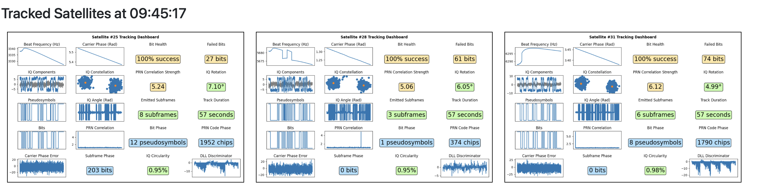
visualizations from this series
 |
 |
 |
|---|
 |
|---|
Table of contents
We can reliably track our satellites over many minutes! We’ve surmounted one of the major challenges in building out gypsum, and now just one obelisk stands before us: computing the user’s position.
This brings us to the really fun part: reading and decoding the bits that these satellites are transmitting!
Unfortunately, this isn’t as easy as I imagined at the start.
Selecting a bit phase
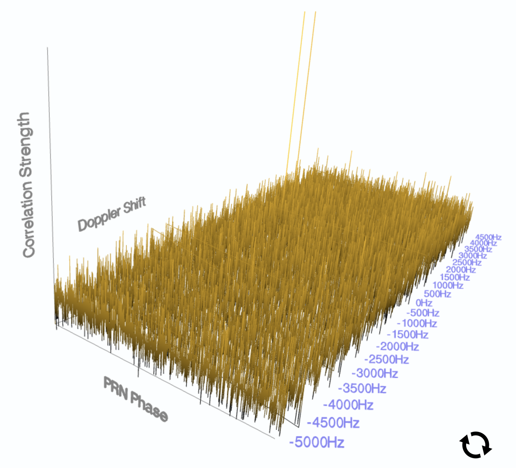
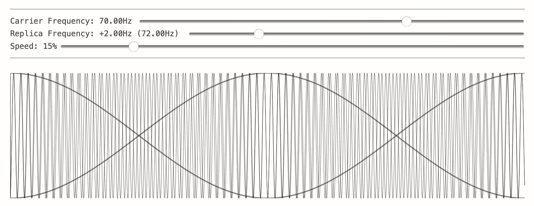
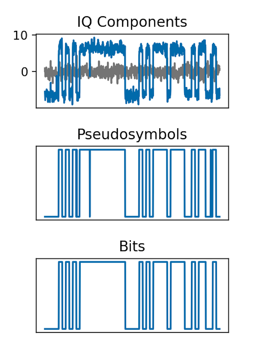
Reading off bits from the satellite requires a peculiar methodology due to the way that the data bits are encoded on top of the PRN code and the carrier wave. When tracking a satellite’s signal, we’ll see a peak each millisecond corresponding to a successful correlation of our replica PRN code with the actual PRN that we’ve read from our radio.
The sign of the PRN correlation itself will tell us the bit value we’re reading✱. If we see a strong positive PRN correlation, the satellite is transmitting a 1. If we see a strong negative PRN correlation, the satellite is transmitting a 0✱.
✱ Note
✱ Note
I’m slightly simplifying, and there’s an interesting challenge here. Depending on exactly when the receiver starts listening to the
satellite, either 1 will correspond to a positive PRN correlation and 0 will correspond to a negative PRN correlation, or 1 will correspond to a negative PRN correlation and 0 will correspond to a positive PRN correlation.
There’s no way for the receiver to know which ‘direction’ the bits are facing without further help. This is called the ‘phase ambiguity’. To resolve this, the satellites send a ’training sequence’ every 300 bits, which is a specific and defined sequence of 1’s and 0’s. When the receiver starts decoding bits, it’ll first look for the training preamble with the bits facing one way, then look again for the bits facing the other way. One polarity should show the training sequence at exact 300-bit intervals (and at some other random intervals, since the sequence can also appear in the message data by chance).
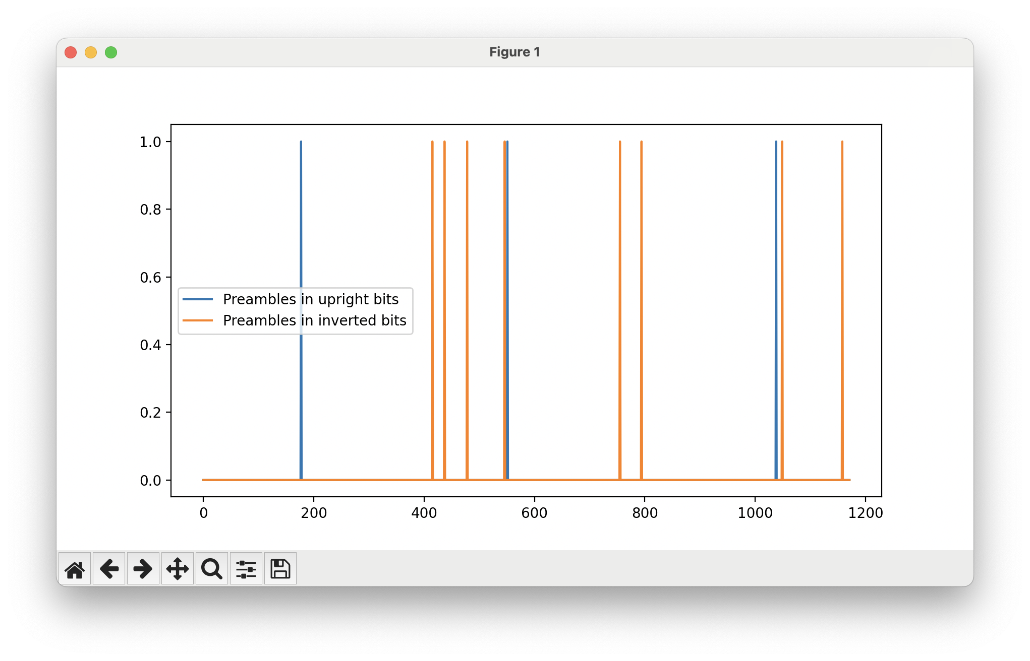
The receiver then selects that as the ‘correct’ polarity, and interprets all the bits received from the satellite with the chosen sign.
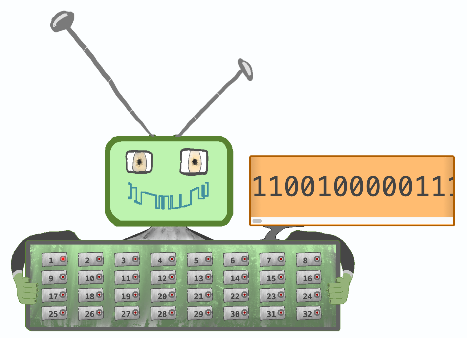
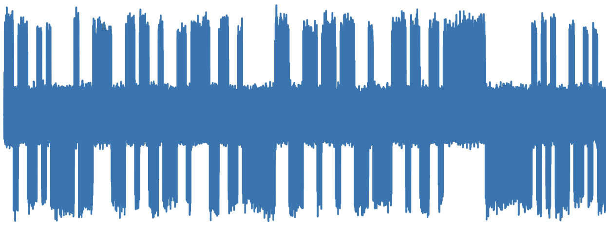
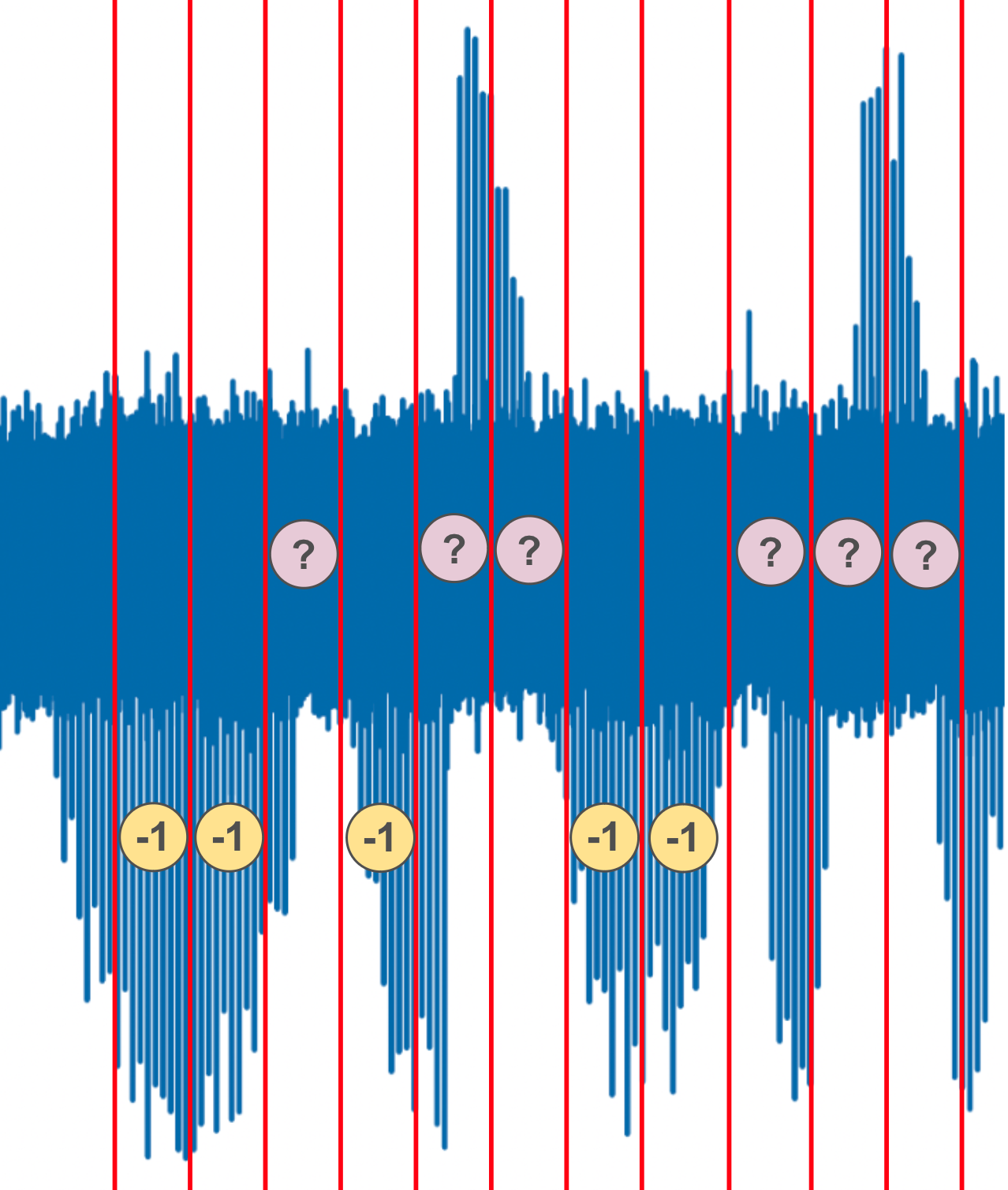
Since we have 1,000 PRN correlations per second, but the satellites only transmit 50 bits per second, we’ll see 20 PRN correlations per bit. Each PRN correlation’s sign isn’t a bit in-and-of-itself, but is instead 1/20th of a bit. Each of these tiny slivers of a bit is called a pseudosymbol, and our receiver will need to aggregate groups of 20 pseudosymbols and decide whether that bit is a 1 or a 0.
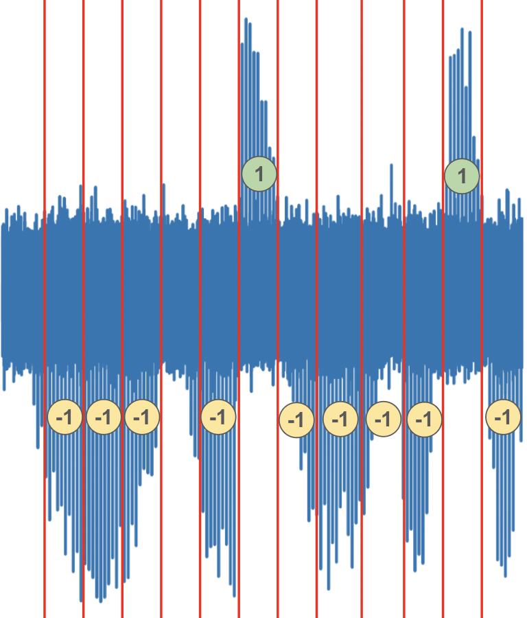
It isn’t too easy to group chunks of 20 pseudosymbols into individual bit values. It might seem obvious when looking at the photo above: just look at when you have a group of PRN correlations all facing in the same direction!
There are practical issues that make this difficult to achieve, though. We might have started listening to the satellite halfway through one of these pseudosymbol groupings. If we just chopped every 20 pseudosymbols, our bits would look really messy and unstable.
Therefore, we’ll need some kind of strategy to detect the edges of the bit transitions. This strategy should also be able to react to change, as our pseudosymbol directions might fluctuate while our underlying satellite signal tracker hones in on the best parameters over time.
I started out with an approach where I try out all the 20 possible phase shifts for the bit edges, and compute a ‘confidence’ based on how strongly the pseudosymbols agree on a bit value. When was the last time your bit was 60% 0 and 40% 1?
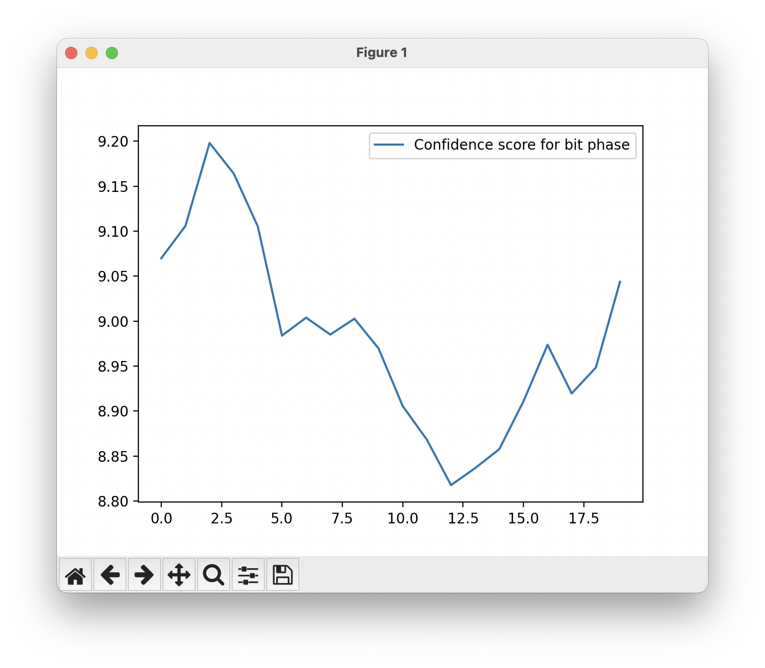
This wasn’t nearly good enough. I had no way to react to change over time. If the tracker takes some time to find the right parameters, but we selected a bit phase that looked good early on by chance, we’d be stuck with an incorrect choice indefinitely. I tried hacking around it by recomputing the best bit phase every half a second, but the approach was fundamentally flawed. We need to dynamically adjust the bit phase as pseudosymbols are processed.
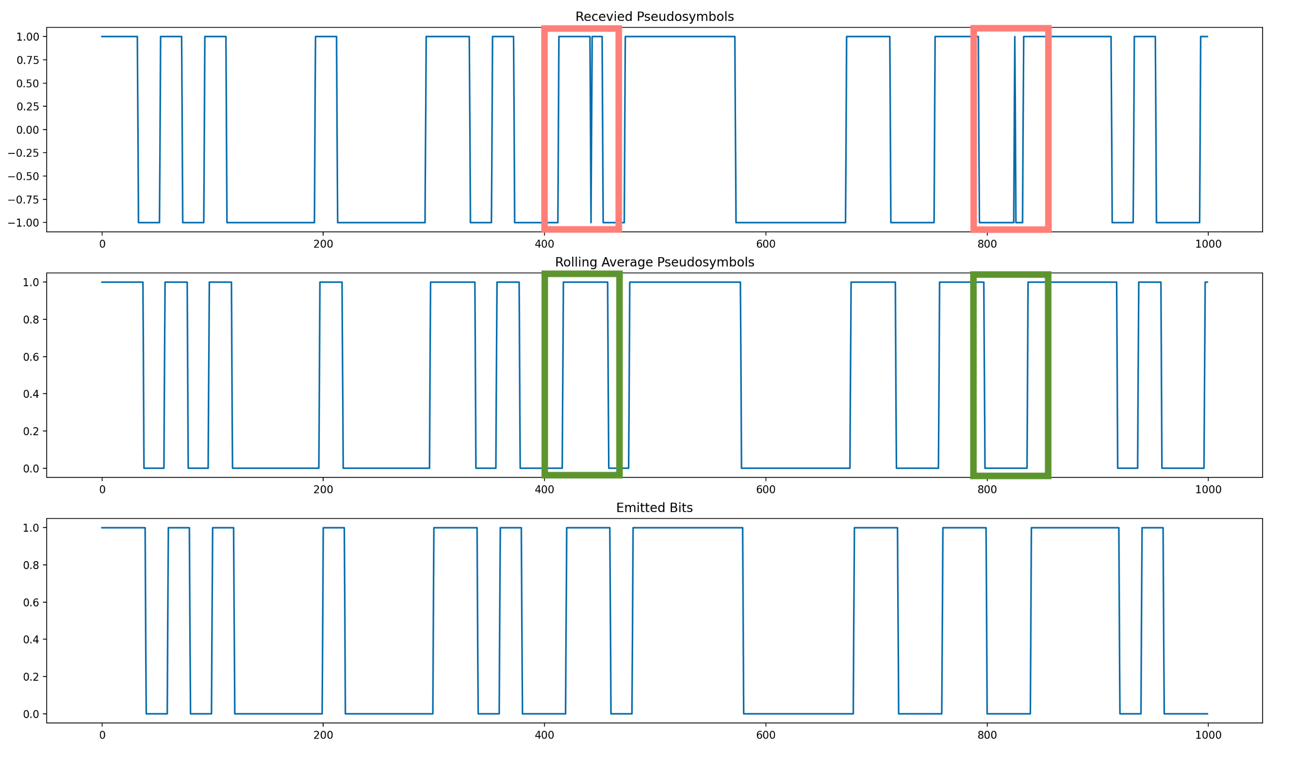
I eventually decided that the best way to do this is to continuously adjust the chosen bit phase as pseudosymbols are processed. I’m keeping a small history of the last pseudosymbols we’ve processed, which allows me to rewind in the pseudosymbol history if we eventually decide that some recent pseudosymbols are actually part of a future bit.
I also implemented a rolling average so that spurious pseudosymbols facing the ‘wrong’ direction for the overall bit get filtered out as a sort of high-frequency noise.
Event pipeline
It’s getting a bit unwieldy to develop our fledgling GPS receiver, and it’s time to rethink its structure. In some ways, writing a GPS signal processing pipeline is a lot more like writing a web service backend than it is like systems programming.
Normally, when implementing a CPU-bound program, you can sketch out a structure in which you have a big block of input data, you apply some series of transformations, and you’re left with some processed output data.
Processing the GPS signals is not like that! For starters, you don’t have all the data upfront. We need to integrate data over time as the antenna data rolls in, and only take action once we’ve accumulated enough context to do something at a higher level. It’s a bit similar to a backend with many scheduled jobs firing off at unpredictable times, as a second-order effect on top of actions undertaken by API users.
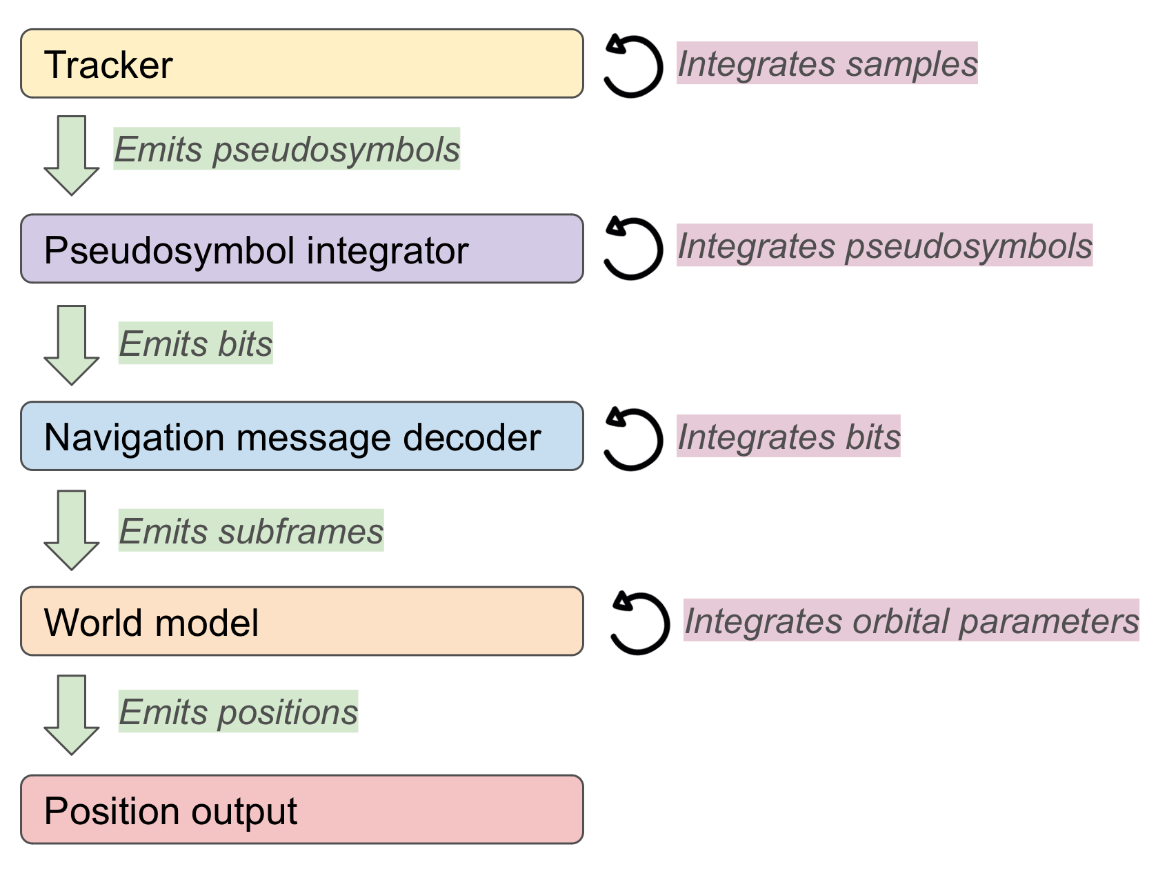
I restructured gypsum to reflect this reality. Instead of trying to keep everything in serial control flow, I switched to an event-driven pipeline architecture. The high-level structure looks something like this.
Timing the signals
Fundamentally, the concept of GPS is that the receiver will keep track of how long it took each satellite’s signal to arrive✱. There’s only a couple of places a receiver could be to have observed the precise arrival times that it actually sees✱, and therefore these arrival times define the user’s position.
✱ Note
This design is encoded in physical realities of GPS. For example, the GPS satellites orbit quite far from Earth: 50 times higher than the ISS. This isn’t a benign choice: the satellites need to be far enough away so that the differences in their signal transmission times are measurable by the receiver!
The GPS designers were brilliant.
✱ Note
There are exactly two position solutions to each set of satellite timing measurements. You can visualize these two solutions by imagining that the GPS satellites all sit along a plane. One solution will be to the left of the plane, and one solution will be its exact mirror to the right.
Typically, the ’left half’ solution will be on Earth, while the ‘right half’ will be the same distance away, but facing out into space. GPS receivers will typically throw away the ‘right half’ solution, implicitly assuming the user is not in deep space.
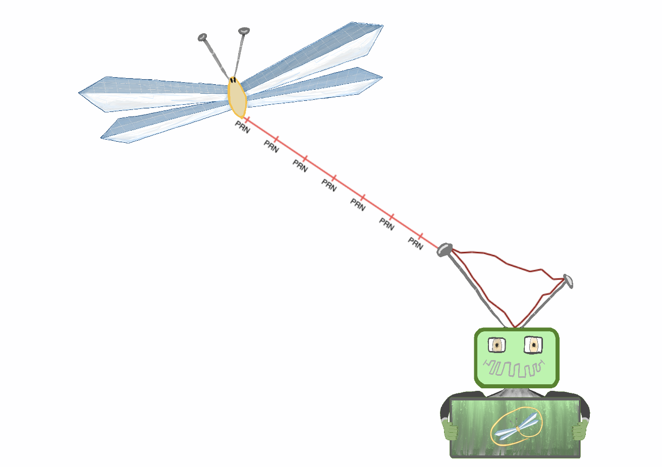
Each satellite will continuously pulse out PRNs each millisecond, providing a nice and stable 1kHz clock tick to any receiver in view✱.
✱ Note
For GPS, though, an entire millisecond is an eternity✱! Thankfully, the receiver can pay close attention to how much of the next PRN has arrived at any given moment, which gives us the precise time delays from each satellite that we’ll need to compute our position solution.
✱ Note
At heart, the only things the satellites say are “Here I am, and here’s what time it is”. Everything else is a geometric derivation by the receiver. This means that the receiver has a huge responsibility: it must precisely handle timestamps of everything that happens, and must be meticulous in calculating and propagating all time material correctly.
All the queuing, shuffling, and averaging that our pseudosymbol-to-bit integrator relies on is antithetical to precise timings. Thankfully, the code changes to affix timestamps to everything that happens in gypsum’s stack aren’t particularly arduous. It was, however, intellectually demanding to correctly figure out how to consider and account for how the structure of gypsum itself, and its various levels of internal queues, affected the observed timestamps down the line✱.
✱ Note
One really fantastic aspect of GPS despite the crucial importance of accurate timings, any delay you introduce doesn’t really matter as long as it’s the same delay for all the satellites.
You can go wild thinking of these esoteric sources of clock calculation error: processing delay in my software receiver, internal queueing, the Python interpreter, the delay between the signal being heard by my RF antenna, processed by my hardware, and delivered to the USB stack… but as long as all of your measured satellite timings are affected in the same way, you can just roll all of them into a ‘global clock error’ term that the GPS position solution will solve away. It’s mind blowing.
I spent several days poring over incorrect position solutions, trying to hypothesize about how this queue or that might cause me to see one signal a fraction of a millisecond faster than another.
Before our grand finale to eliminate these pesky mistimings, let’s take a look at exactly what these satellites are beaming down.
The navigation message
“Here I am, and here’s what time it is”. Doesn’t sound too bad, right? Before we dust our sleeves off and call it a day, it’s worth remembering that the payload was specified in the 1970’s, for use on 1970’s era space hardware.
The mechanism by which each satellite describes its position is quite involved✱. Bits are at a heavy premium in the navigation message, so much of the logic is offloaded to the receiver itself.
✱ Note
The mechanism by which the current time is described is quite involved, too. You might wonder how the satellite communicates the current time when the message itself has to be sent over time at a 50 bits per second data rate. The satellites actually don’t send the current time, but send the timestamp of the first PRN correlation of the next satellite message, each of which takes 6 seconds to transmit. It’s remarkably well-timed: the satellite is spending exactly 6 seconds to say “at the end of this 6 seconds, the current time will be X”. By the time the receiver has heard the final piece of the message, it’s precisely the time mentioned in the message.
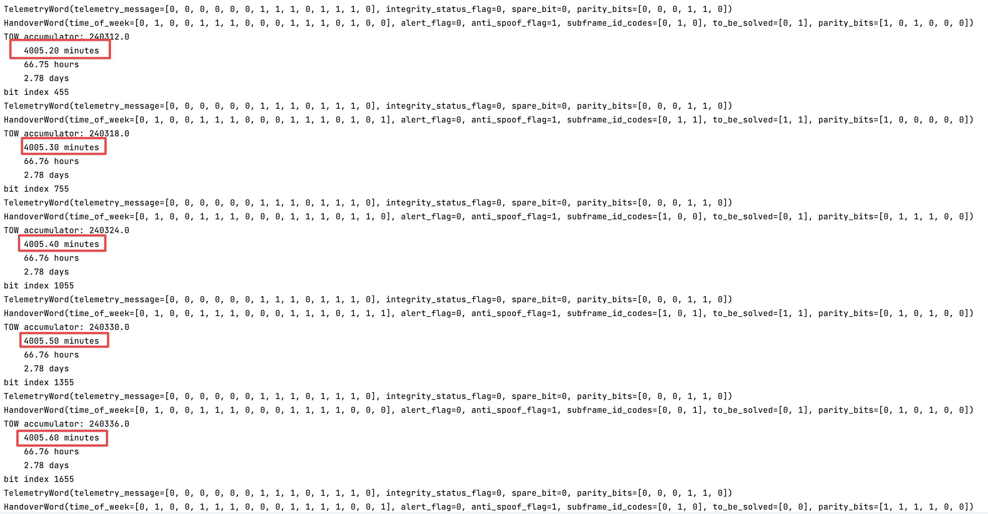
The time format is also bespoke. GPS doesn’t use UTC but its own timescale instead, with its own epoch and no leap seconds✱. This means that every GPS receiver in the world that outputs times needs to hard-code how many leap seconds have elapsed so far, so times can be converted back to UTC. Not just that, but GPS also undergoes its own 2038-type problem every 20 years, as its ‘current week’ counter rolls back to zero.
Along the same lines, GPS timestamps are typically expressed in “seconds since the start of the week” to save space. The specification then encodes special-case calculations for using GPS in the few hours at the end of every week and beginning of the next.
✱ Note
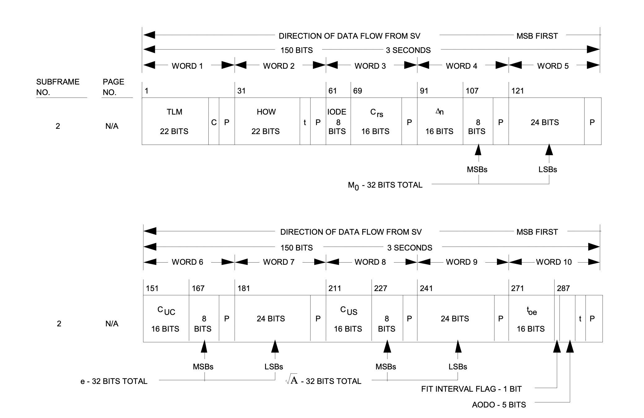
In particular, the satellites don’t describe their actual positions. Instead, they send orbital parameters that describe how the satellite’s position at a given time can be computed from certain orbital equations.
But not just that: these orbital parameters need to be stuffed into a small and compact message, so even they need to be derived by the receiver. The satellite will send the high 8 bits of an orbital parameter in one field, a low 24 bits in another field, and these fields need to be combined and multiplied by 2 x 10e-16 to get the true value. Another will contain the square root of the true orbital parameter. It feels more like bit-banging a hardware driver than communing with an atomic clock shooting by in outer space.
I parsed the navigation message and retrieved the orbital parameters, but it’s nigh impossible to spot-check whether these values look reasonable by just glancing at their magnitudes.
Luckily, there’s an intuitive way to check whether a set of orbital parameters seem sensible: plot the orbit!
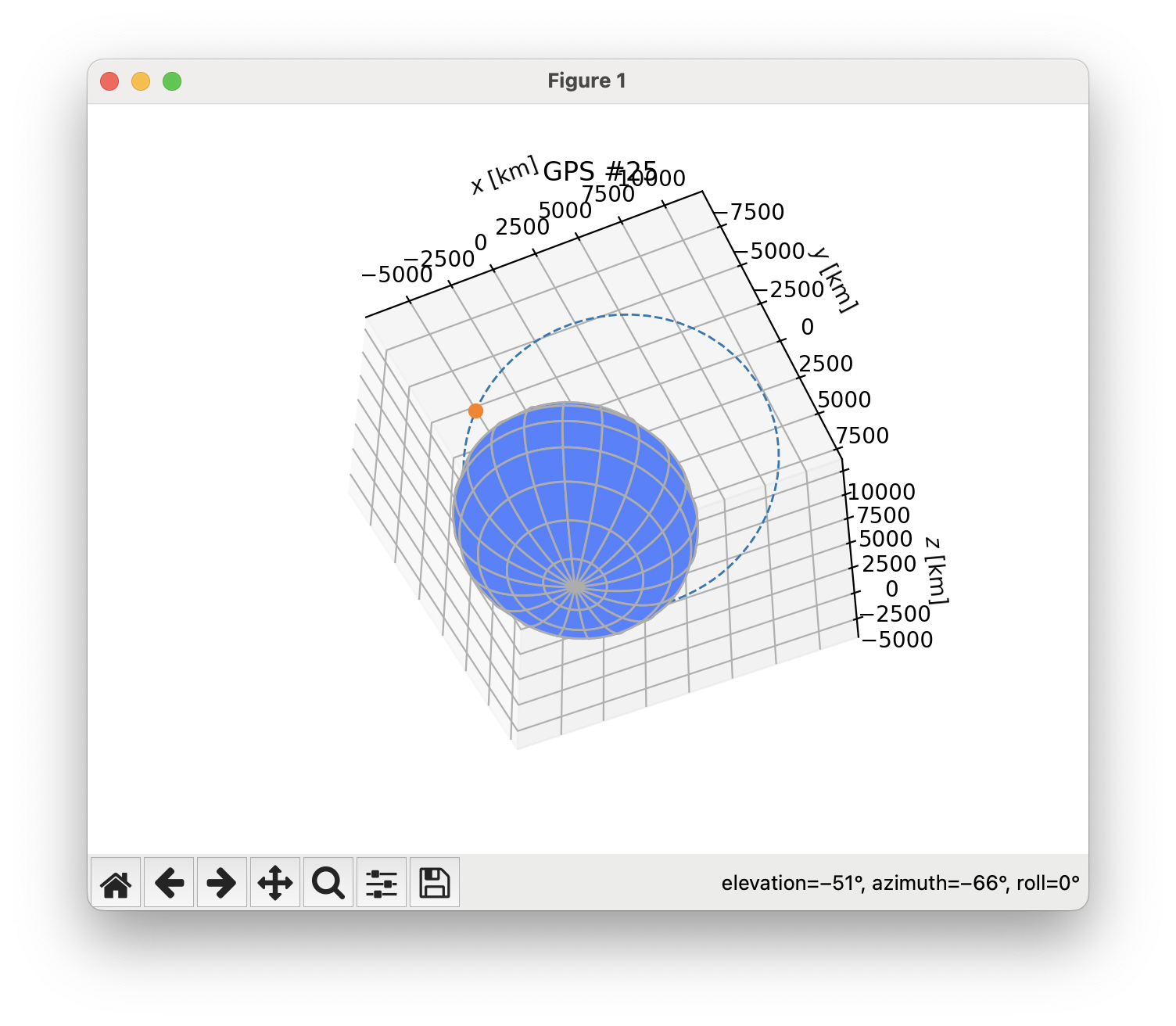
Hmm. Our first reading of the satellite’s orbit shows that the satellite is due to crash into the Earth in the next couple of hours. This is… probably not correct. Read more in Part 4: Measuring Twice.