Building a GPS Receiver, Part 1: Hearing Whispers
Reading time: 11 minutes
In this 4-part series I build gypsum, a from-scratch GPS receiver.
- ↳ Part 1: Hearing Whispers
- ↳ Part 2: Tracking Pinpricks
- ↳ Part 3: Juggling Signals
- ↳ Part 4: Measuring Twice
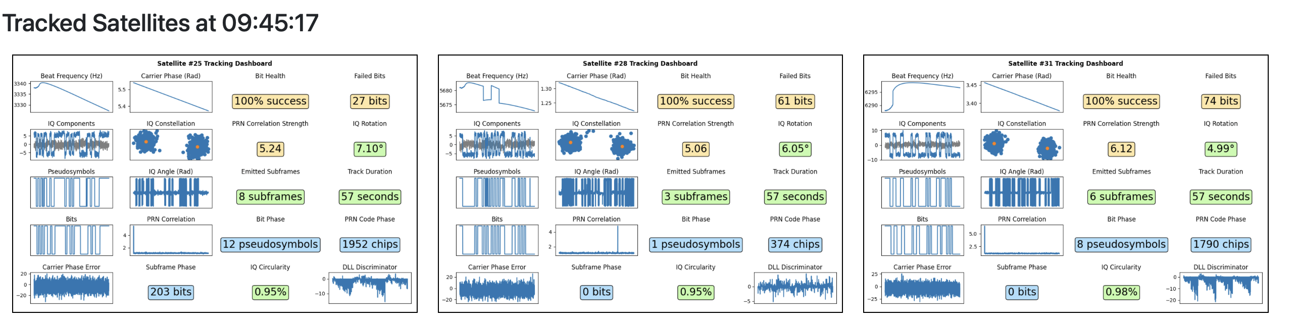
gypsum's web dashboard
visualizations from this series
 |
 |
 |
|---|
 |
|---|
Table of contents
Introduction
✱ Note
Have you ever noticed that your Maps app still works during a flight? It can feel illicit, like someone just forgot to turn off the signal, and that watching yourself crawl along the earth should be done without drawing undue attention.
A few months ago I learned that there were only around 30 GPS satellites serving the entire planet. This piqued my interest, because it reminded me of the 13 root DNS servers from which all resolution flows. Perhaps GPS has a similar design in which the ‘source of truth’ is diluted by several layers of signal repeaters?
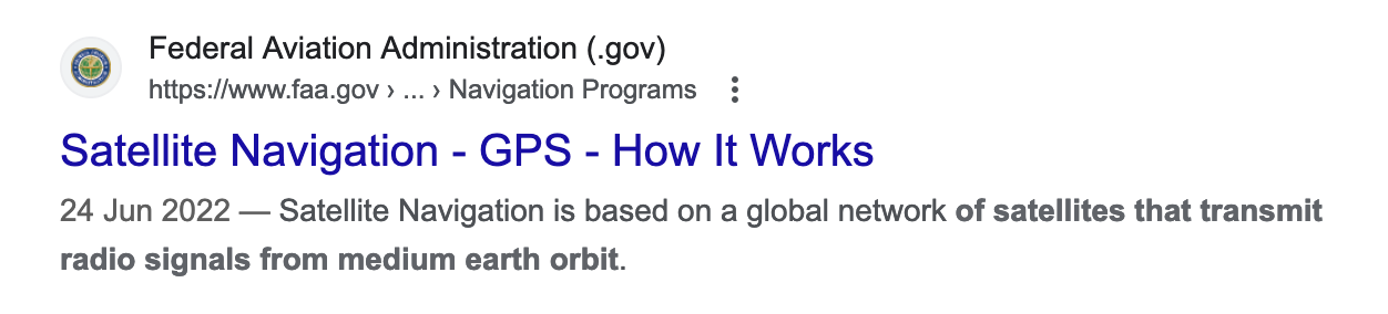
I navigated to gps.gov, and was presented with this delightful image. I became even more excited to learn about what these satellites do!
I decided to try my hand at decoding these GPS signals, guided by the vague end-goal of plucking out my position from peanuts.
I learned that the GPS signals that facilitate our mapping apps are ever-present, around us at any altitude, in any weather conditions, at all times.
This sounds cool in the abstract, but the tangible reality is staggering. These signals are all around me as I write this. They’re all around you as you read it. The world is soaked in these whispers, repeating themselves endlessly for anyone willing to listen.
You can find out exactly where you are, from thin air, anywhere at any time, by learning to speak the language of the electromagnetic waves flowing over your skin. These waves have been a constant and quiet companion for most people’s entire lives✱.
✱ Note
GPS is perhaps one of the most audacious geo-engineering feats ever undertaken, and its traces can be felt with just an antenna and a motive.
Quiet beacons
All that said, it’s not as though there’s a cacophony of navigation data swarming around you, deafening if you could just hear it. In reality, the GPS signals surrounding you are astoundingly weak. To take an analogy: imagine a normal light bulb, like the one that might be above you now. Pull it twenty thousand kilometers away from the room you’re in, and have it flash, on, off, on, off, a million times a second. Imagine straining your eye to watch the shimmer of the bulb, two Earths away, and listen to what it’s telling you.
Big reveal: this is not hyperbole! The signal pumped out by GPS satellites actually has the same strength as a residential lightbulb at the satellite. By the time the flash gets to you, it’s unfathomably attenuated, and yet it can still be detected, decoded, understood and made useful. It’s really incredible, and hard to believe without wrangling the data yourself.
These quiet lighthouses give rise to one of the interesting characteristics of GPS: there’s no way for anyone to charge for access to it. No one even knows you’re listening. From the satellite’s perspective, GPS is send-and-forget✱.
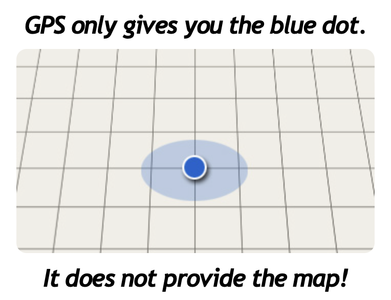
Similarly, your GPS location could never be served up to you by a web service. The key idea with server-side computing is that compute might need to be served in one place (such as on a user’s machine), but it’s really no problem if it’s computed in another (such as a data center). GPS, by contrast, is fundamentally incompatible with this optimization: GPS only tells you about the radio waves hitting where you are, and you need to listen to what’s in the field around you. No datacenter can listen on your behalf.
Listening closely
OK, you’ve got me, I’m pumped! How do we, uh, listen?
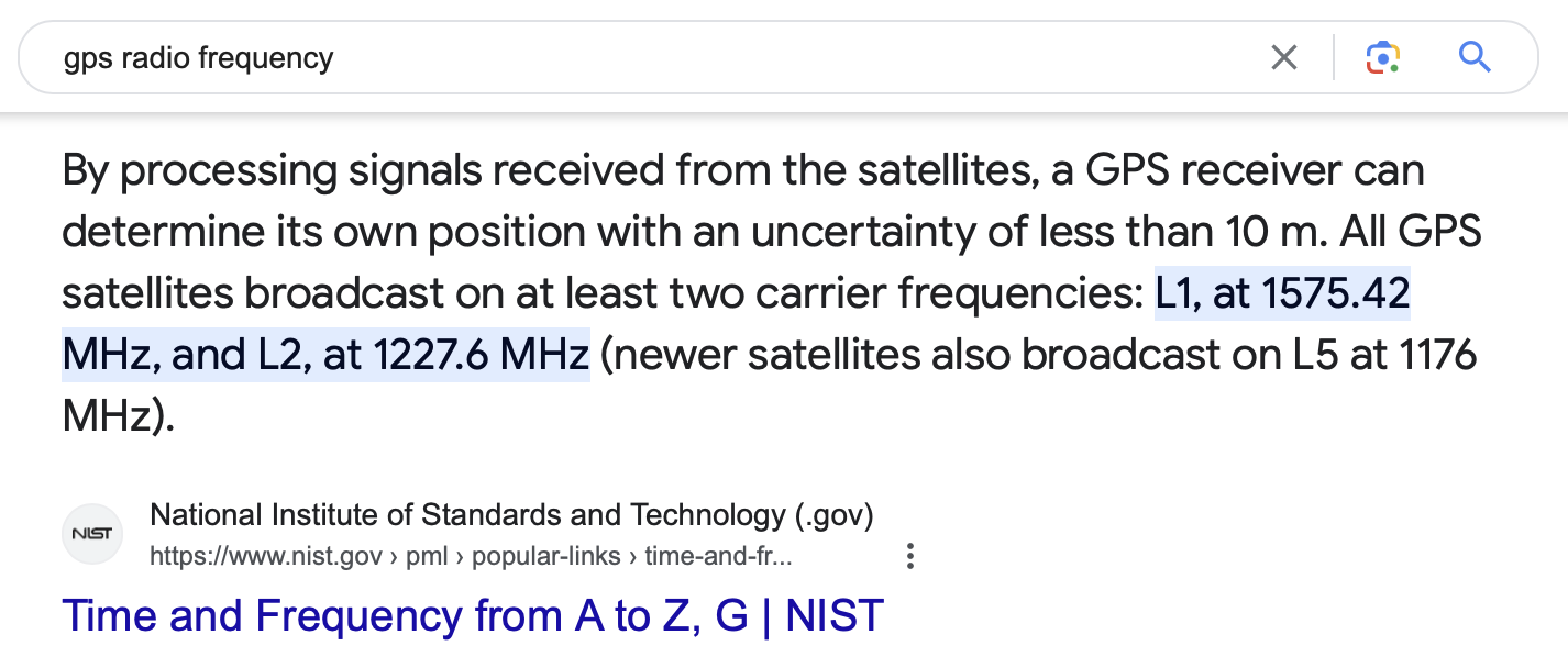
I understand that GPS is transmitted over EM waves, but I don’t know much about the analog domain – is this the same thing as radio?
Great! I know that frequency is important, where does that come in?
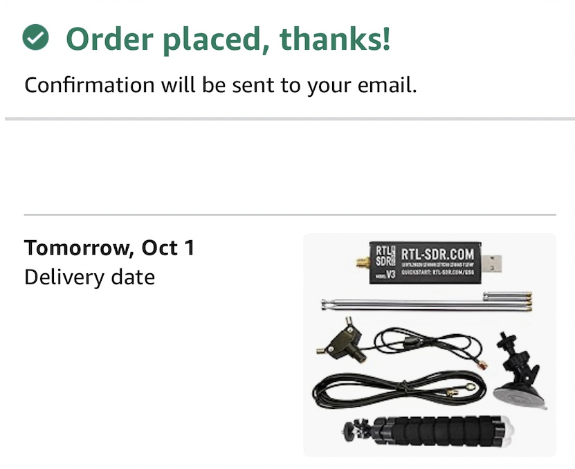
Cool. I know I’m going to write some software to receive these signals, post-process them, and make a snazzy demo for my pitch deck. I figure this means I’ll need to buy a receiver that can tune to the GPS frequency. After searching around for a tunable RF receiver, I learn that I’m looking for a ‘software defined radio’. This sounds reasonable!
I hastily research SDRs and purchase one just before my flight takes off.
I set up SDR++ and start poking around. For a while, I can’t find much of anything, but after speedrunning terms such as bias tee✱, AGC✱, and IQ correction✱, I’m ready to go to town exploring the spectrum.
✱ Note
✱ Note
✱ Note
SDRs output ‘IQ samples’. I refers to the in-phase part of the signal, and Q refers to the quadrature (or imaginary) part of the signal. My understanding is that this scheme allows you to process the signal in “3D” (time, amplitude, and polarity) instead of just in “2D” (time and amplitude).
Due to the circuitry of an SDR, there’s a large frequency spike at whichever frequency you’ve asked the radio to tune itself to. This can be quite confusing as a beginner, as it looks like there’s a strong signal anywhere you choose to look! Although this spike is an unavoidable artifact of how the SDR functions, there are a few ways to remove it from your collected data. One of these is to tune the radio slightly ’to the side’ of the frequency you’d actually like to measure, so that the center spike isn’t polluting your real signal. Another, which is a bit less fiddly, is to use some software to detect and try to remove this spike at the centered frequency. This feature is called IQ correction, presumably because it works by mucking about with the IQ samples before delivering them to the rest of the stack.
Locking on
By the time it’s received by terrestrial antennas, the GPS signal is so weak that it has 100,000 times less power than the ambient energy and signals just floating around the place. In other words, the GPS signals can sit up to 50db below the thermal noise floor✱.
✱ Note
The newer GPS satellites are meant to send signals that reach receivers at around -130dBm. The typical residential thermal noise floor at the C/A bandwidth is about -110dBm.
For comparison, cell signals are around -50dBm: 100 million times stronger than the GPS signal!
Our signal has been entirely swallowed up by random perturbations far stronger than the signal we’re trying to detect. It seems obviously impossible, then, that any data could be recovered.
Incredibly, the GPS signal can be identified and decoded, despite being far below the thermal noise floor. GPS accomplishes this through the use of a clever signal processing technique that allows a signal to be found even when surrounded by noise.
Hearing the inaudible
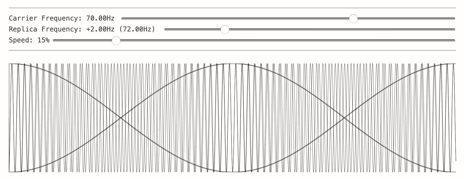
When we’re trying to listen to the GPS satellite, there’s an information asymmetry: the satellite has data that the receiver doesn’t have, and the receiver wants to hear it. However, the receiver cannot hear such an incredibly weak signal in the face of the (comparatively) much louder cymbals and crashes of the random signals floating around the surface of the Earth.
So, GPS uses a trick here. Although there’s unknown data that the GPS satellite sends, we can also have the satellite send a signal that’s known to both the satellite and the receiver. This extra signal, called the C/A✱ code, the PRN code, or the chipping code, is repeated by the satellites a thousand times a second.
✱ Note
C/A stands for coarse acquisition, and it exists in contrast to the P, or precision, code. GPS was initially envisioned for military use, and the C/A code was intended to be a low-resolution stepping stone for military receivers to lock on to the much more precise P code. Nowadays, the C/A code is the basis for most civilian GPS, whereas the P code is still only available for military use.
Interestingly, the only thing stopping civilians from using the P code is the knowledge of the value of its chipping sequence. If the formula to generate the P code was publicly known, there’d be nothing stopping civilian GPS receivers from locking on to it, with the exact same techniques as are used for the C/A code.
Similarly, the only reason the P code is so much more precise than the C/A code is that it operates at a higher chipping rate! As we’ll see later, the exact phase of the code is one of the key observations that allow the receiver to calculate its distance from the satellite, so a code that transmits more frequently inherently gives a higher distance precision.
Since the receiver knows exactly what to listen for here, the receiver can sum the received signal over and over again and compare the actual signal to the PRN signal the receiver is expecting. The noise, being random, will average down to zero over time, while the PRN signal will keep growing and growing✱. This trick is referred to as spread-spectrum. GPS uses a trick-in-a-trick to make this whole thing work with multiple satellites, which is called code-division multiple access.
✱ Note
Now that we have a way for the receiver to hear the otherwise inaudible PRN, the GPS satellites take the PRN code and ‘mix’ the actual data signal they want to transmit into it. While the PRN code operates at a million bits per second, the data signal is transmitted much slower, at 50 bits per second. By keeping the data rate significantly slower than the PRN code, GPS ensures that the PRN code remains a reliable fixture to lock on to for large fractions of a second, while also ensuring that the data stream can be reliably recovered.
Generating the C/A codes
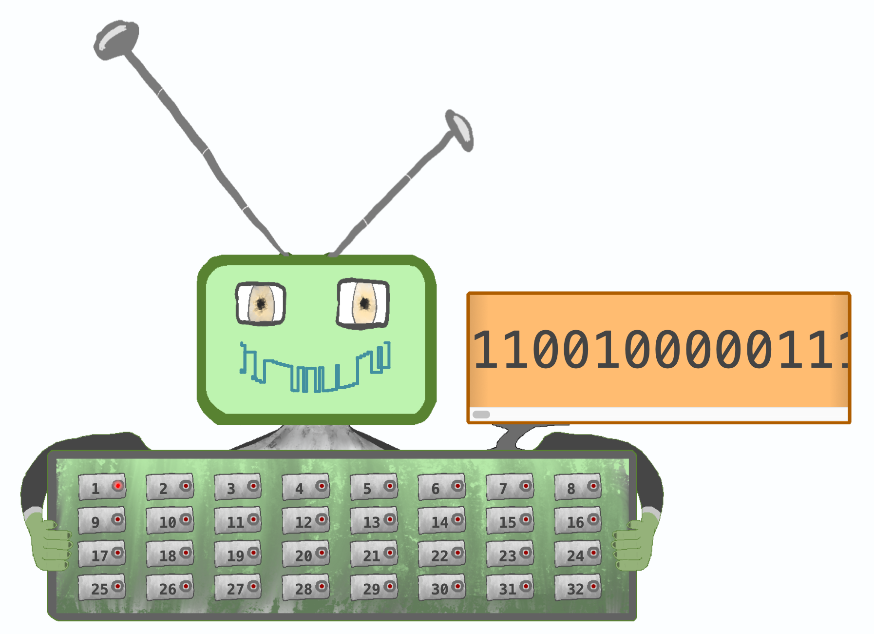
We don’t just have one PRN code, though. There are 30 GPS satellites in the sky, and to achieve our eventual goal of figuring out where we are, we’ll need to know exactly which of the satellites are above us.
Therefore, each GPS satellite has its own unique, stable PRN code.
These codes are described by Table 3-I (Code Phase Assignments) of the IS-GPS-200L, the civilian GPS specification.
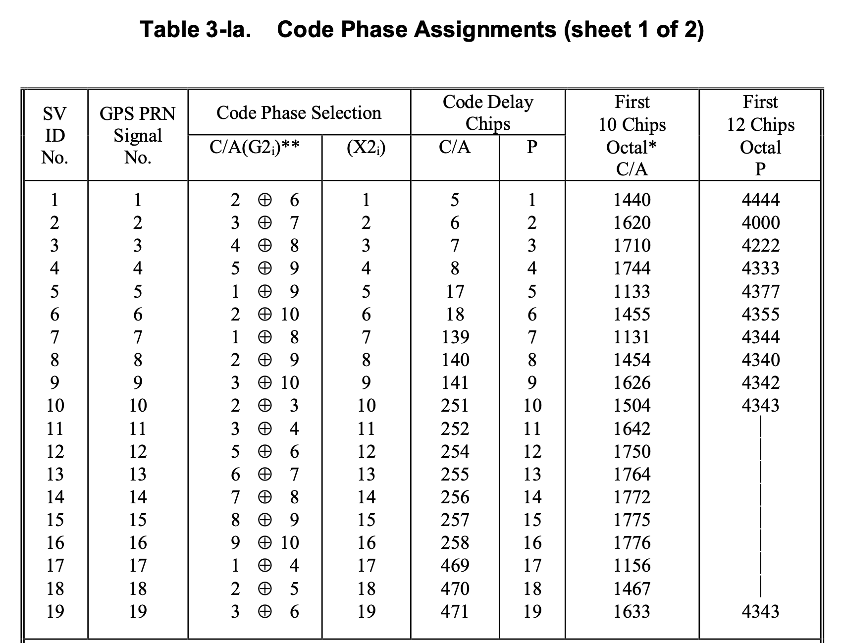
If you search around, you’ll find a lot of resources online telling you how easy it is to generate the PRN codes, and very little by way of actual reproductions of the full PRN codes for you to check against.
These codes are relied upon many millions of times daily, and it makes me wary that I didn’t find them online. I’m leaving them here for posterity. I hope this helps someone!

Acquisition
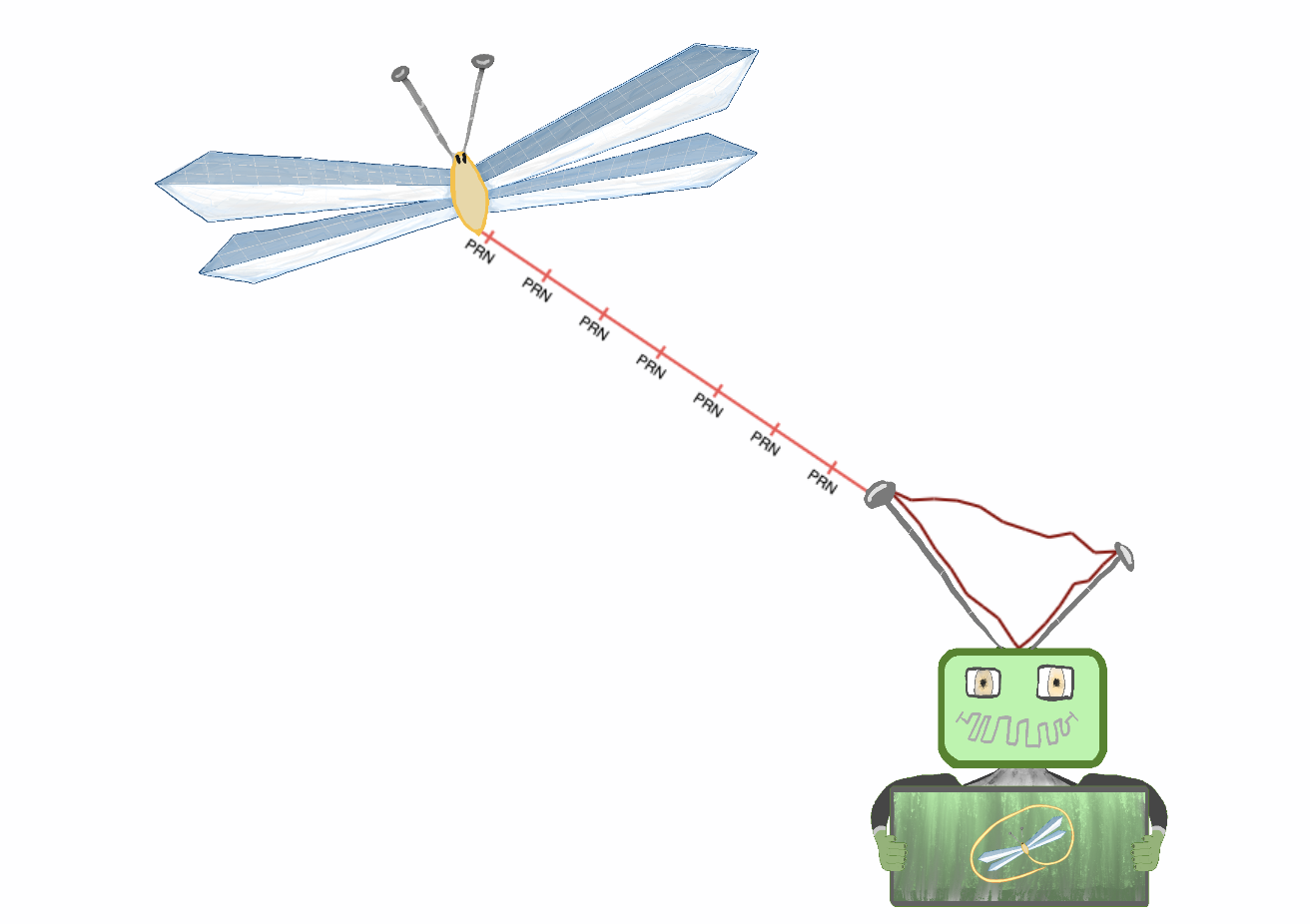
To investigate the sky for the satellites that are in view, GPS receivers need to generate a copy of each PRN that’s being emitted by each of the 32 satellites, then search for each of these PRNs in the data that the GPS receiver is collecting over its antenna. This phase is called ‘acquisition’, because the goal is to ‘acquire’ a lock on whichever satellites are in view above the user.
Our GPS receiver needs to take a short snapshot of antenna data (a second or so will do), and correlate the received data with each of these replica PRNs. If there’s a strong correlation between our replica and the live data, we know that the satellite associated with that PRN is chirping away above us.
However, the signals that reach us aren’t the ‘ideal’ PRNs that we’ve generated locally. Just like the GPS signals are attenuated due to passing through Earth’s atmosphere, other physical effects also impact the signal we receive. Since the GPS satellites are transiting so fast above us, the signal we receive from each satellite will be Doppler-shifted in frequency.
Since the GPS satellites transit at well-known orbital velocities, we know the range of Doppler shifts we’d expect the signal to reach us at: up to a +5KHz frequency increase for an approaching satellite, or -5KHz frequency decrease for a satellite travelling away from us.
Also, since we’ve started listening for the GPS signals at some arbitrary point in time, we might start hearing the PRN halfway through its transmission.
Therefore, when searching the data we’ve received for satellite signals, we need to search across several axes at once:
- Each satellite’s PRN code.
- The range of Doppler shifts that we’d expect the PRN code to be slid by.
- The phase that we’ll slide our replica PRN code by to match up with the received PRN code.
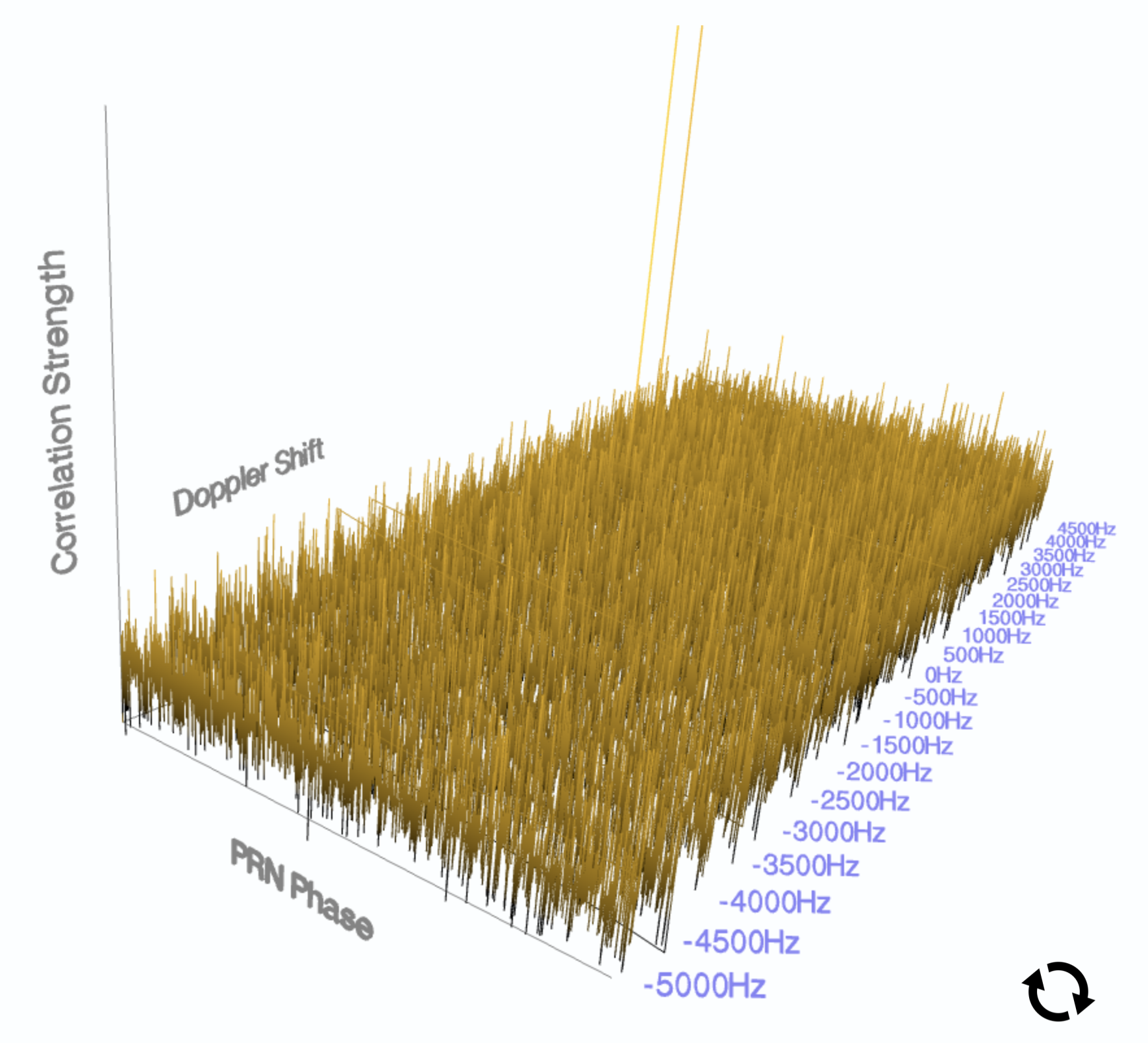
This acquisition phase of the GPS receiver tends to be compute-intensive. Thankfully, when you do stumble on the correct parameters the correlation spike makes things pretty clear!
There’s a wealth of academic papers out there exploring ideas to speed up and optimize acquisition. It’s quite remarkable: some papers are entirely founded on tweaking the equation in effectively one line of code, and exploring how this impacts the acquisition performance characteristics.
I’m transforming each PRN from the time domain into the frequency domain, and correlating the frequencies of the incoming satellite data with the spectrums of each PRN code. This is really useful because a phase offset in the time domain becomes a shift in frequency components, and what that means is that I get to perform steps #2 and #3 in the same computation✱! I’m also using a binary search sort of approach to converge on the Doppler shift that gives the strongest correlation spike for each satellite in view✱.
✱ Note
✱ Note
All said and done, we’ve built a detector to determine which GPS satellites are in the sky above us, as well as a rough approximation of their phase (or time delay), and Doppler shift (or relative velocity). We’ve completed the first major step in the GPS positioning pipeline, and we can now say with confidence which GPS satellites are currently above the user! Read more in Part 2: Tracking Pinpricks.