Building a GPS Receiver, Part 2: Tracking Pinpricks

We’re getting there! We’ve set up a pipeline that can read vast quantities of floating point samples from our radio hardware, and can pick out the hums of the GPS satellites amongst the noise.

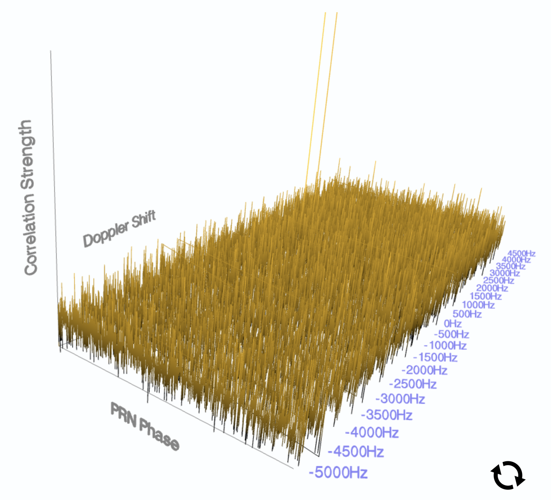
Our acquisition phase told us which GPS satellites are within view of the user, and has given us a coarse estimate of each satellite’s Doppler shift and PRN sequence phase.

However, these satellites are extremely precise devices in a noisy and changing environment, and our coarse estimates won’t nearly cut it.

1. The satellites will continue transiting above us, so their Doppler shifts will continuously change over time.
2. The signals might be impacted from time to time by atmospheric obstructions.
3. Our own radio’s hardware relative inaccuracy will cause our replica PRN signals to drift from the satellites over time.
4. The user might move positions or change their velocity.

Our tracking phase will painstakingly follow each satellite’s signal as they change over time. We’re going to take a quick pit stop to dig into what the signals we’re detecting from the GPS satellites really are.

The carrier wave

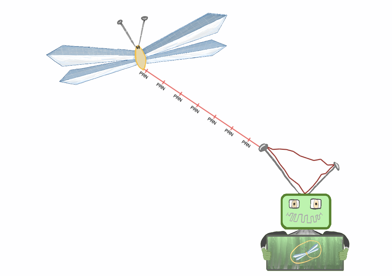
We know that we’re plucking the satellite’s PRN out of the static heard by our radio by generating a ‘replica’ PRN, then searching for that replica at various Doppler shifts and phase shifts. But satellites don’t just transmit a PRN, in the abstract. Instead, the PRN sequence, and all information transmitted by radios in the general sense, is transmitted on top of a carrier wave.

Just like the GPS satellites will mix the navigation data as a low-frequency perturbation of the PRN, so too is the PRN a perturbation of the fundamental unit transmitted by any radio transmitter: a sine wave. This sine wave ‘carries’ any information transmitted by a transmitter. To transmit information, the transmitter applies some modification to its sine wave^✱.

This sine wave defines the frequency of the transmission. When we say that GPS transmits at 1575.42MHz, we’re saying that its carrier sine wave oscillates 1,575,420,000 times per second. When your favorite radio station is at 97.2MHz, it means that all the audio transmitted by that station are vibrations relative to a carrier sine wave oscillating 97,200,000 times per second.

To hear the transmitter’s modifications to the carrier wave, we’ll first need to precisely lock on to the carrier wave emitted by each satellite.

Just one problem: you won’t find any SDR on the market that will claim to be able to sample a wave oscillating over a billion times a second. At best, you’ll find SDRs with a sampling rate of about 40MHz, suitable for sampling a sine wave of 20MHz^✱. Our GPS carrier sine wave, vibrating well over a billion times per second, is light years beyond what any SDR can sample. And yet, of course, GPS trackers are everywhere. What gives?

The beat wave

As it turns out, no GPS receiver is sampling the carrier wave directly.

Instead, any time you ask any radio to tune to a given frequency, what the radio will do is internally generate its own ‘replica’ carrier wave at that frequency. This is similar to how our GPS receiver will generate replica PRN codes matching what we expect to be emitted from the satellite. The radio will automatically ‘mix’ anything it hears with this replica carrier wave that the radio has generated, allowing the radio to be more sensitive to perturbations around this frequency^✱.

Since we have a coarse estimate of the satellite’s Doppler shift, but not an exact measurement, the replica carrier wave that we generate will be close, but not exactly matching, the carrier wave that we truly receive from the satellite.

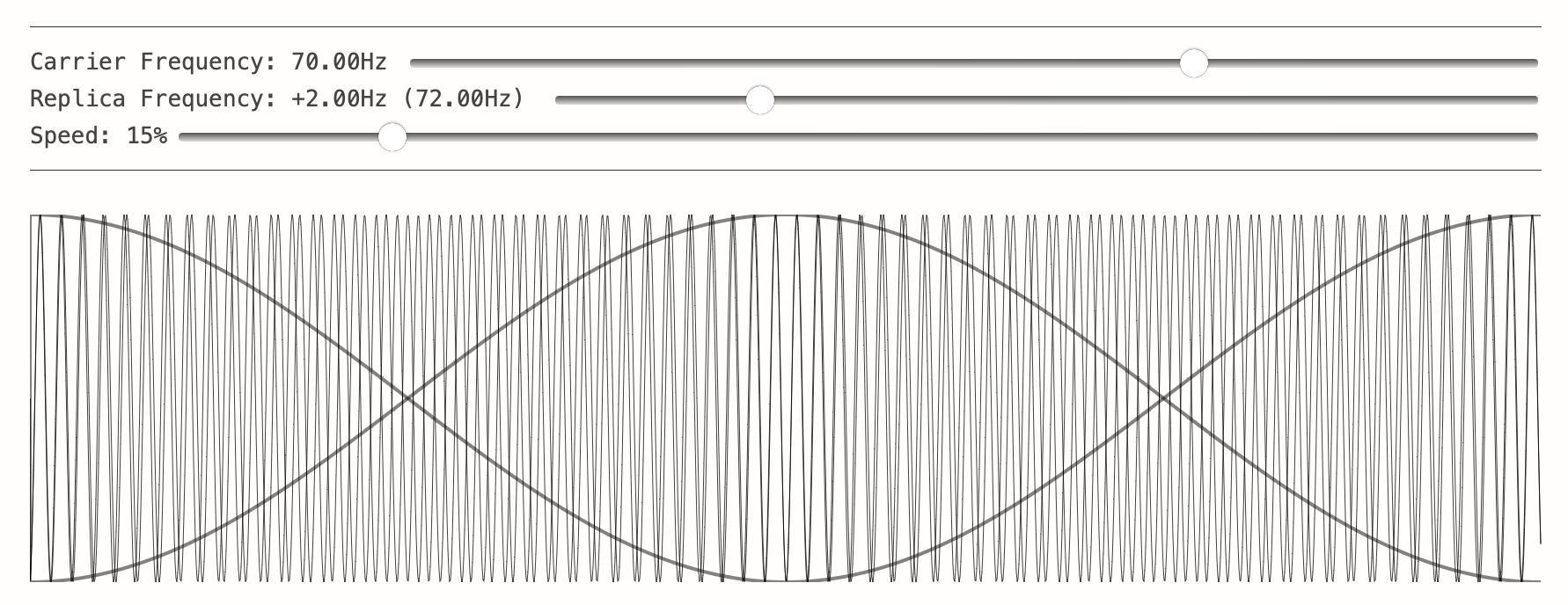
Two sine waves close in frequency, but not exactly matching, will create a beating wave. It’s actually this beating difference that GPS receivers track when trying to hone in and maintain hold on the carrier wave^✱!

There are some really neat properties that can be observed in the visualization above.

Firstly, the difference between these two waves is exactly the difference in frequency between our replica carrier wave and the true carrier! Locking on to the beat frequency tells us the precise frequency adjustment we need to make to our replica carrier to line things up perfectly with the incoming signal.

Secondly, it doesn’t matter how fast the underlying frequencies are oscillating! Try dragging the Carrier Frequency slider back and forth. The difference in frequencies (the ‘helix’) will look exactly the same, and its shape is governed only by the difference in the two waves.

Lastly, notice how the beating wave is a lot more difficult to pick out with your eyes once the offset between the two waves exceeds 8Hz or so. This is exactly the challenge that the GPS receiver faces too: if our estimated replica carrier wave is more than a few Hertz away from the true incoming carrier, it’ll be too tricky for our tracker to identify and lock on to the beat frequency.

Now that we have a foundation for how we can hone in on the carrier wave, we’re ready to build our tracker!

Tracker control loop

To eventually decode the bits the satellites are transmitting, we’ll need to painstakingly track:

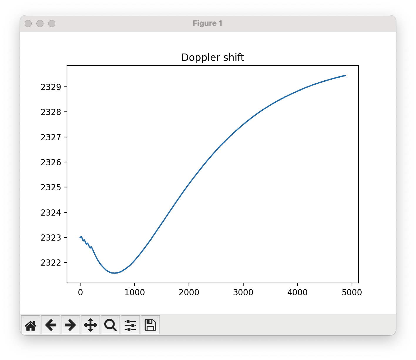
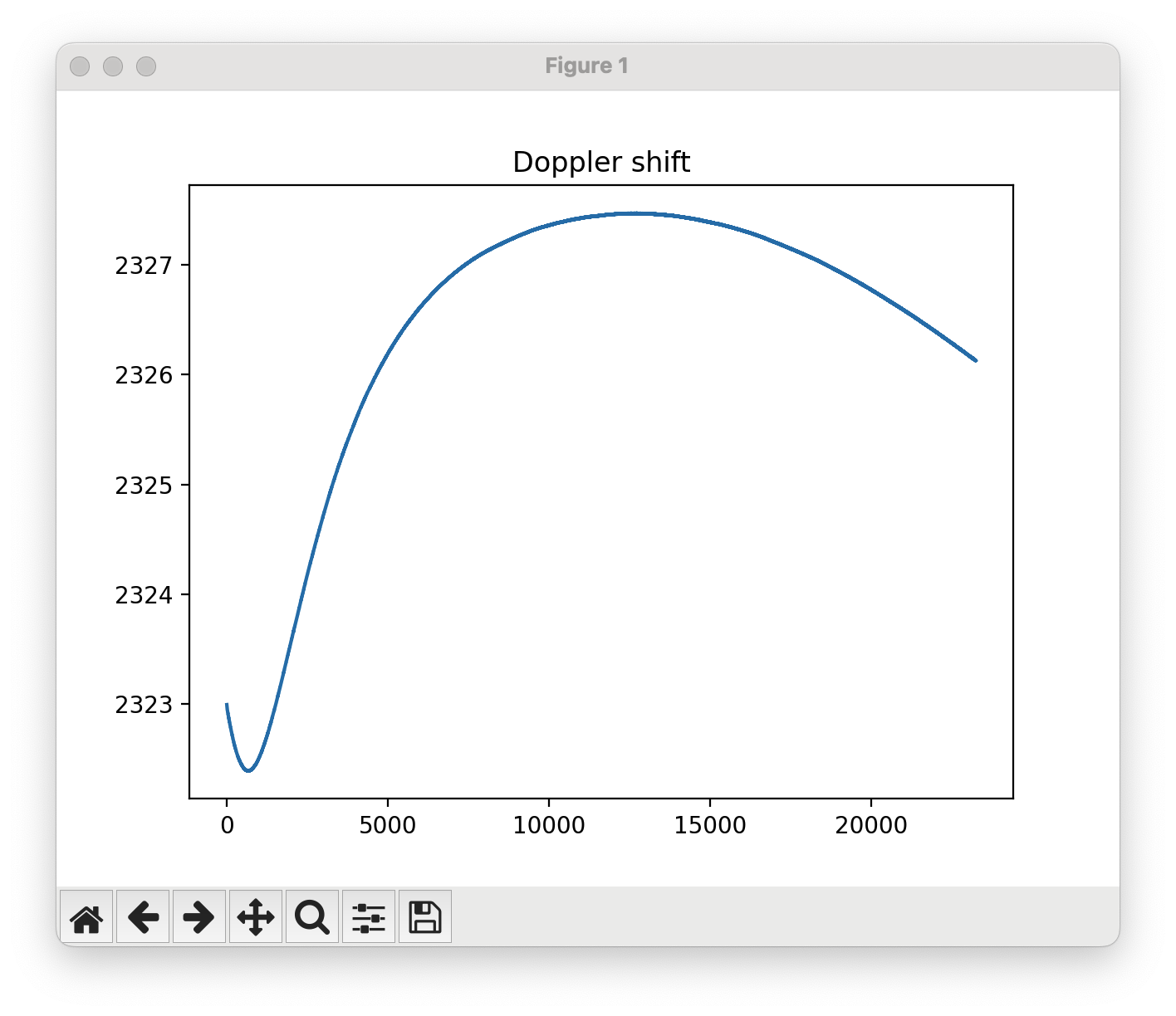
1. The Doppler shift of the satellite signal.
2. The received carrier wave phase.
3. The received PRN code phase.

We’ll need to make minute adjustments to our estimations of these three variables to stay locked on each satellite. To do so, we’ll dip our toes into control loop theory: we need to be able to react to errors instantaneously, but also be able to integrate a correction over time. We need to accomplish both of these goals without being too slow to react to changes, or too fast that we jitter our way out of a locked state.

This took me a couple of weeks to get working, which was particularly painstaking because it’s hard to tell you’re on the right track at all until you have a finished and working control loop. Signal processing is really hard.

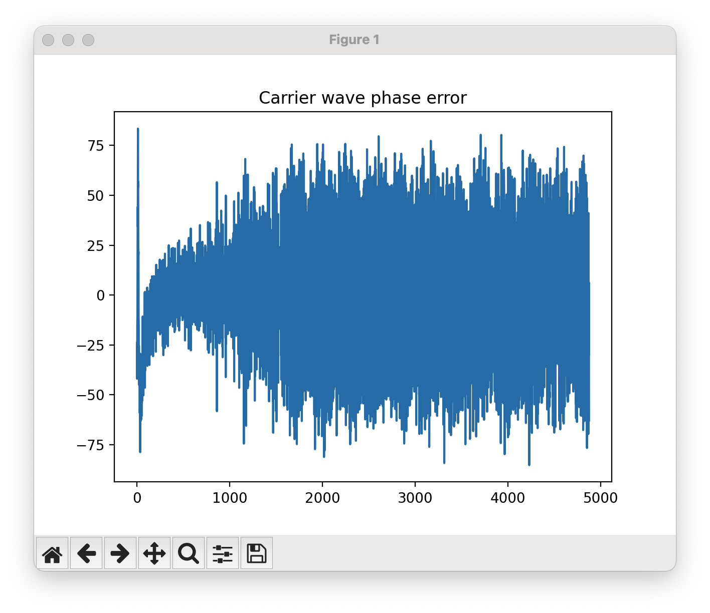
You can tell when you’re not locked onto these variables correctly because your estimations will be, simply put, all over the place.

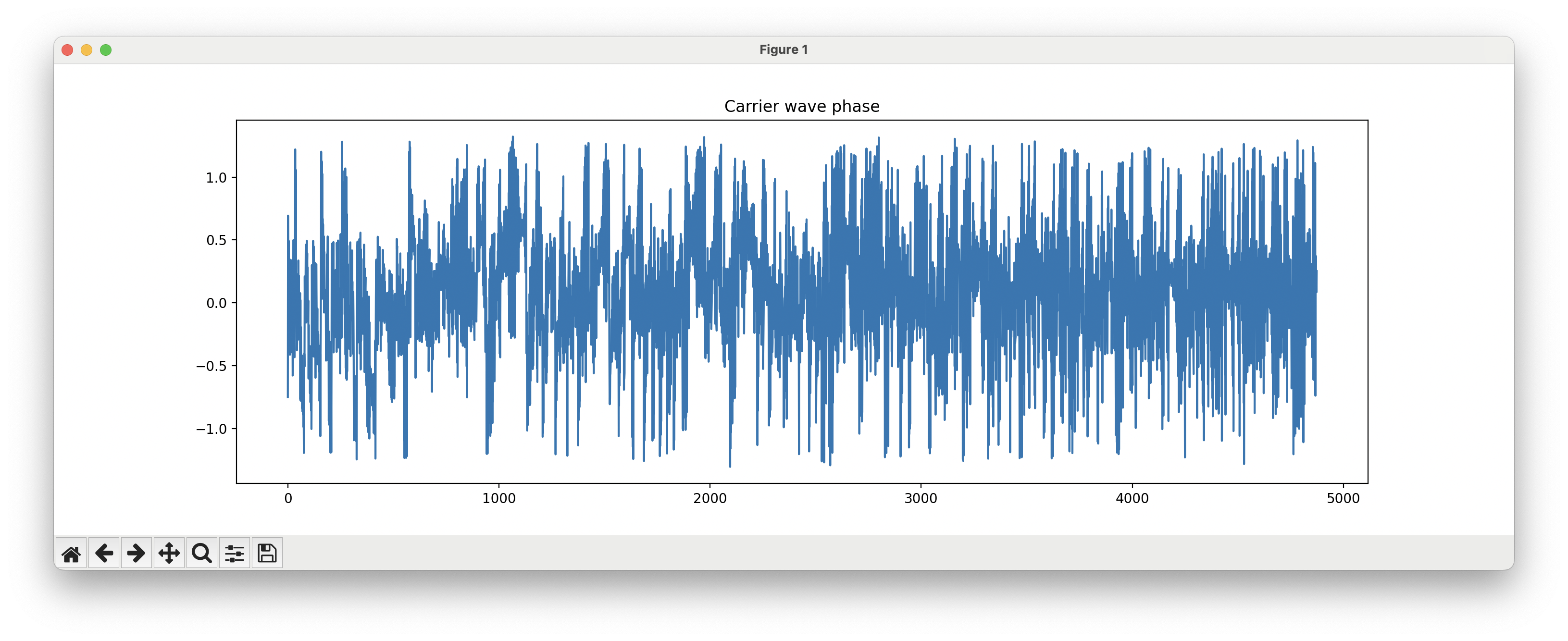
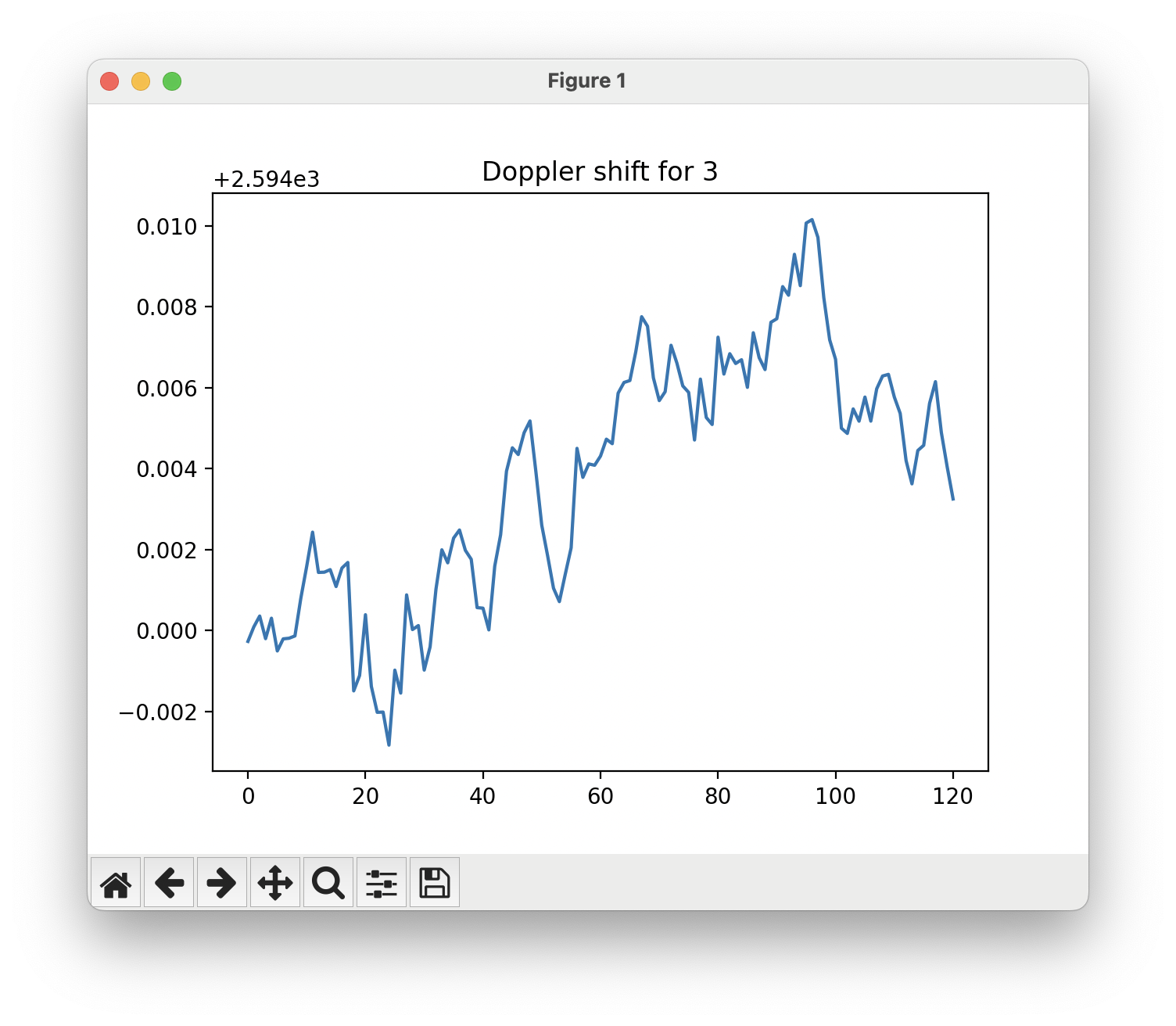
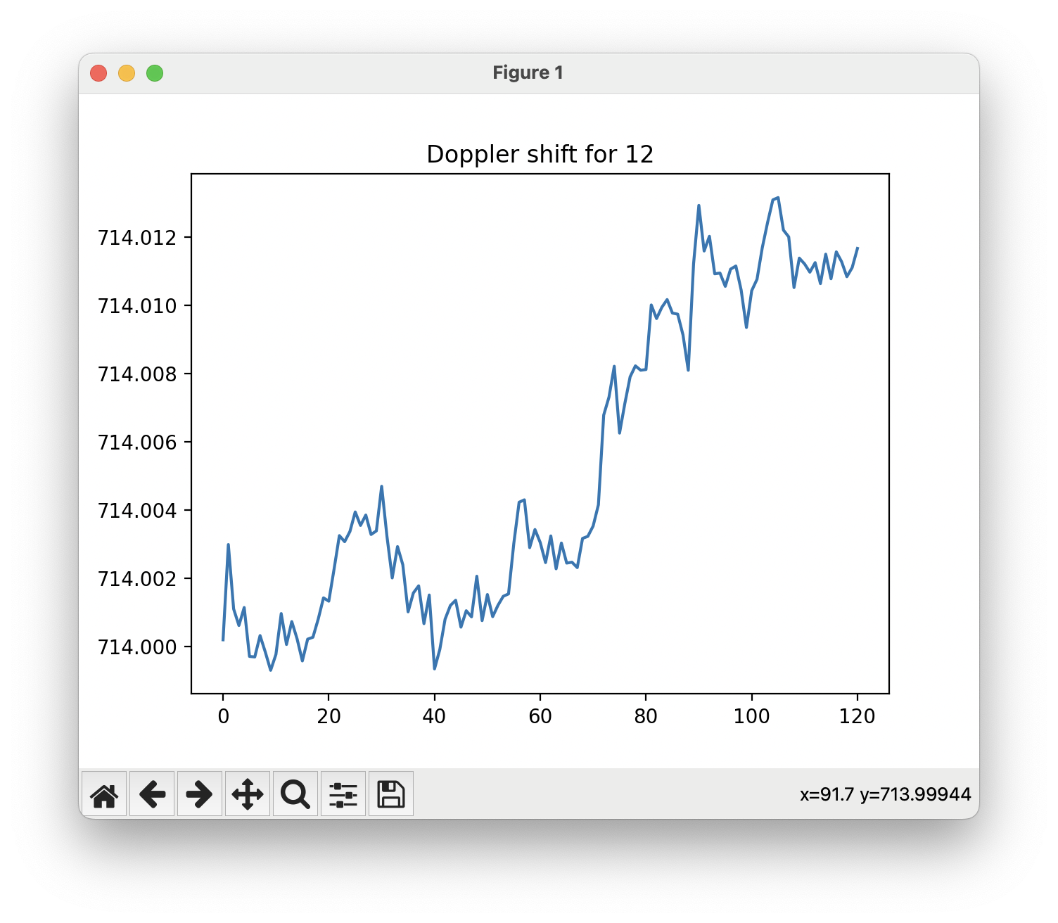
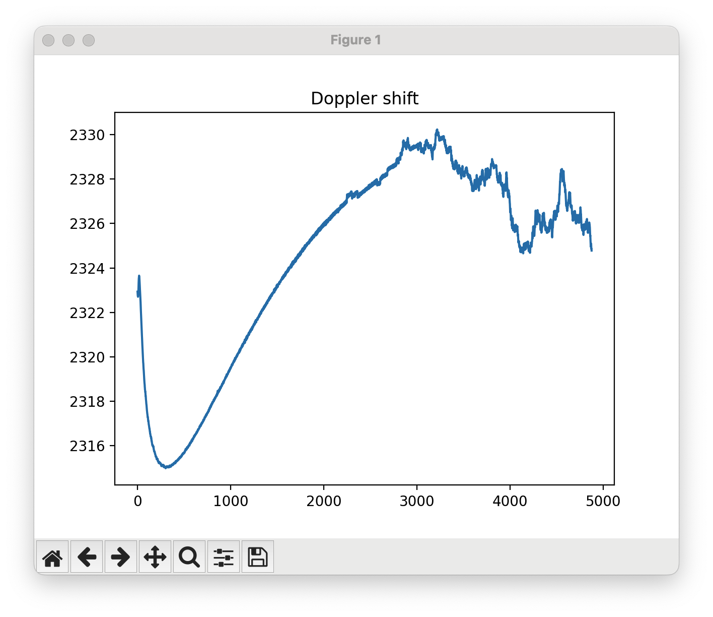
But once you do get it working, you’ll be rewarded with these beautiful, smooth tracking curves that stay resolutely fixed on the physical reality of the signal over time.

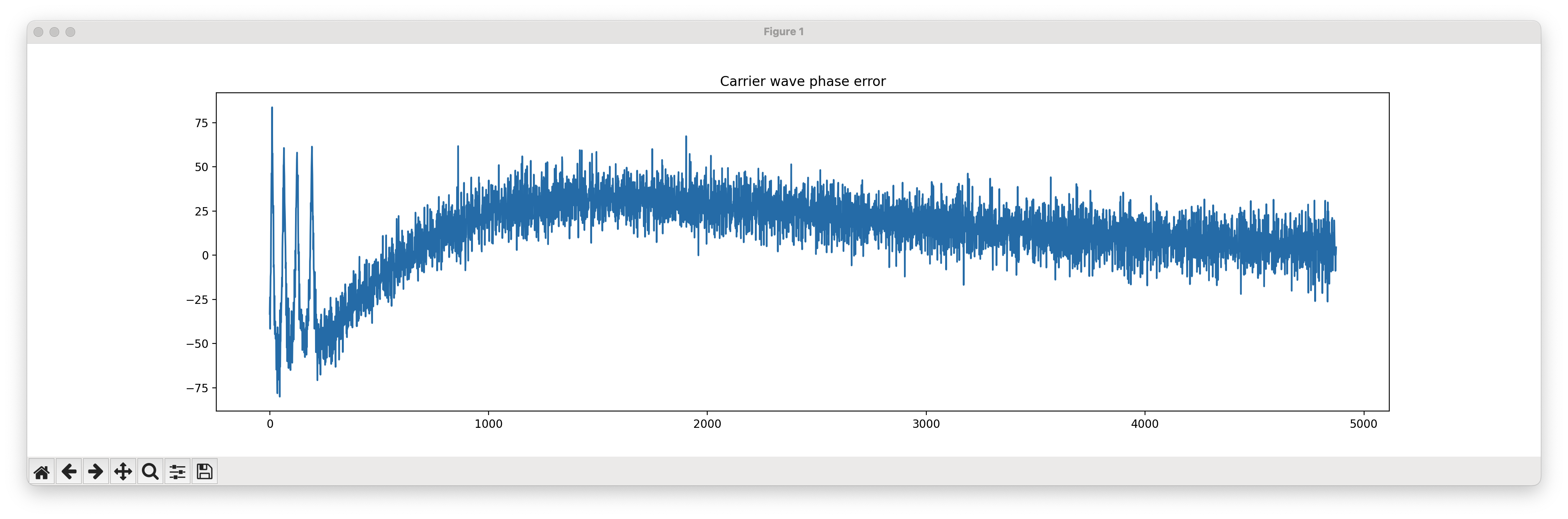
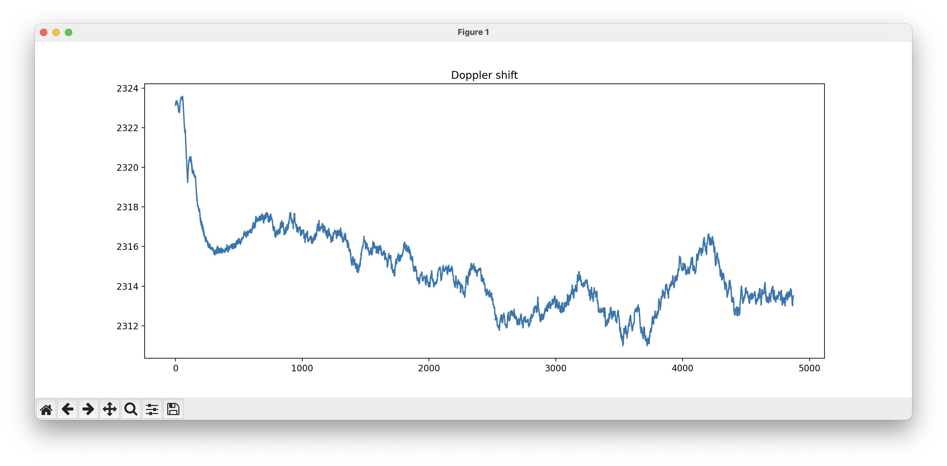
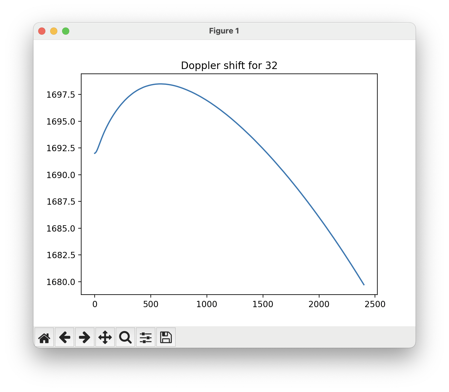
Without a good strategy to react over time, you might start out with decent tracking, then devolve as the signal characteristics change.

In hindsight, a good tracker was the most difficult part of building a GPS receiver by far. I ended up having to deviate quite severely from the standard approaches.

Rebellion

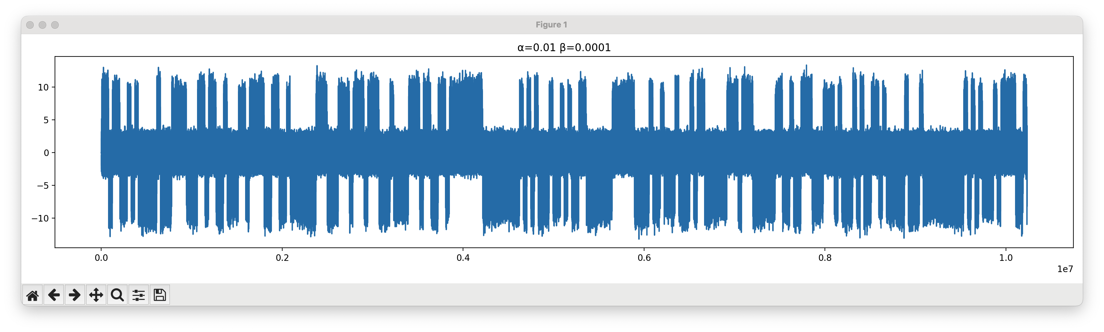
The standard GPS literature is exceedingly clear on how the tracker is supposed to work: you use a delay-locked-loop (‘DLL’) for tracking the shift of the PRN’s starting point, and a phase-locked-loop (‘PLL’) for tracking the phase and frequency of the carrier wave. A GPS receiver’s PLL typically uses a technique called a Costas loop^✱, and all of these control loop techniques are controlled by use of a couple values called the loop filter coefficients. There’s a delicate balance to be struck: keep the loop filter coefficients too small and the PLL will never find the correct parameters, but increase the coefficients too much and the PLL will start tracking random noise instead of the signal of interest. It’s generally understood that, with enough tenacity and caution, you will be able to find coefficients that strike the right balance.

I built a small interactive widget that allowed me to modify my loop filter coefficients in real time as my signal was processed.

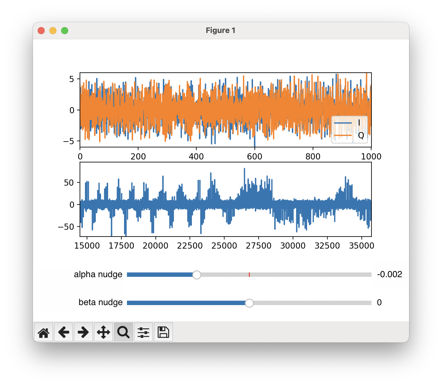
In my case, it wasn’t possible to find a single pair of coefficients that could track a real-world signal for more than a few seconds. After weeks of hoping and tinkering, I eventually had to garner the courage to just sit down with the signal and implement something that works.

Before I can figure out how to adjust my PLL, I need to understand exactly what’s happening with my signal processing across a bunch of different dimensions. The real breakthrough was creating this signal processing dashboard that allows me to dissect exactly what the demodulated signal looks like, instead of trying to glean everything from the pretty Doppler curves.

I ended up augmenting the traditional PLL with a few strategies. These made it possible for my receiver to track real satellites over the course of many minutes.

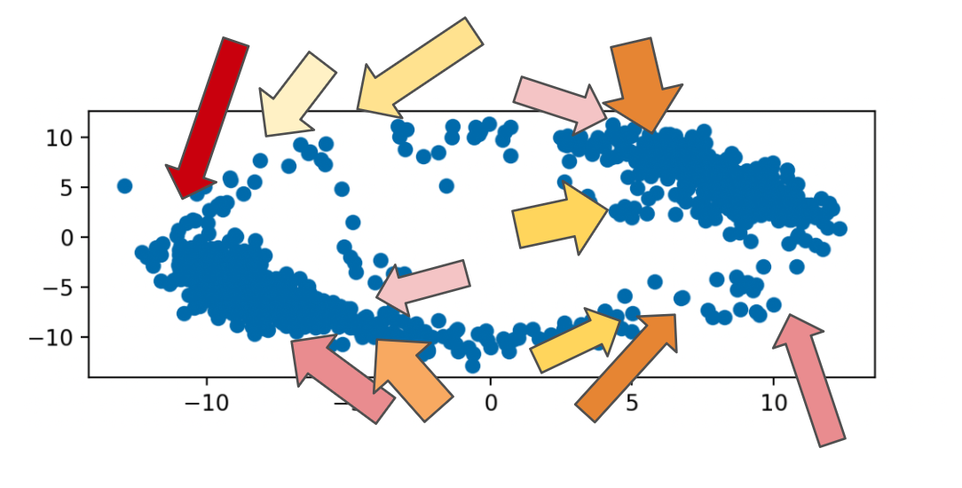
Tracker gadget #1: Constellation twister

One of the new insights granted by the visualizer was that the IQ constellation^✱ occasionally exhibited a rotation.

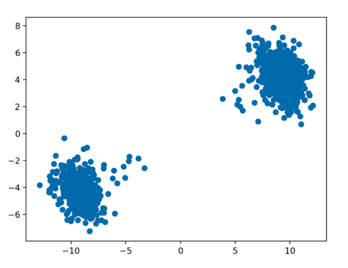
When the PLL is faithfully tracking the carrier wave, our demodulated IQ constellation will look something like this:

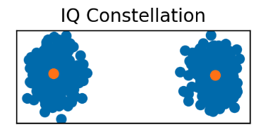
Two blobs locked to the X axis.

When the PLL is off and our demodulation starts to go hairy, our demodulated IQ constellation might look like this instead.

Wouldn’t it be nice if we could just twist the constellation to get things back on track?

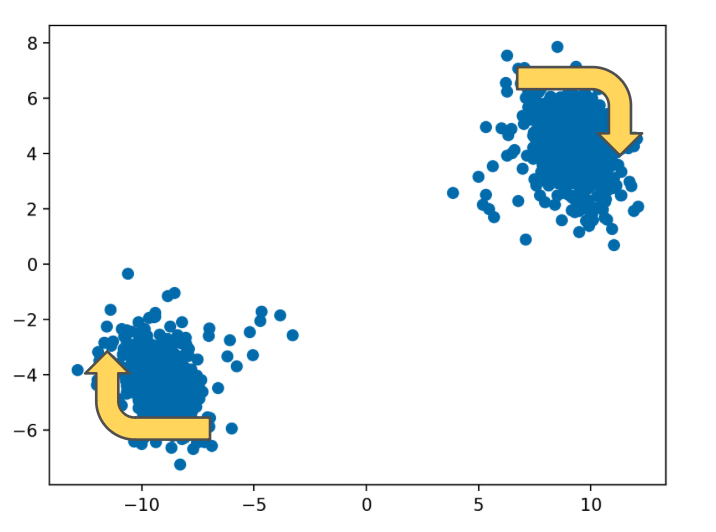
I added a periodic job that runs every few seconds, examines the ‘rotation’ of the blobs, and applies an upwards or downwards frequency correction to try to align the blobs horizontally.

This was laughably effective. It single-handedly took me from the realm of losing satellites after mere seconds, to several minutes of robust satellite tracking.

Tracker gadget #2: Constellation groomer

Similarly, when things are going poorly, our two IQ blobs are instead smeared out into a circle^✱.

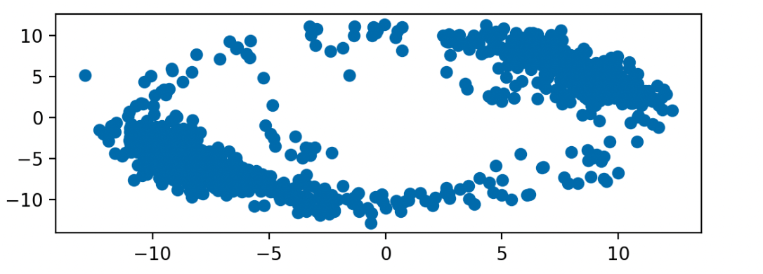
I added another job to inspect the ‘circularity’ of the IQ plot, and to apply a correction if the two blobs were getting a bit too friendly with each other.

Tracker gadget #3: Decision-directed maneuvers

One difficulty is that observing a smeared constellation plot tells you that your carrier wave estimation is wrong, but it doesn’t tell you how it’s wrong. The frequency estimation could be too high, too low, or the phase estimation could be incorrect^✱, but all of these issues will result in the same sort of visual perturbations in the graphs.

I ended up adding a mechanism that attempts both increasing the carrier wave frequency estimate, and decreasing it, then choosing the direction that results in a better looking plot.

By using these techniques and more, and by burning through years of stored patience, I was able to build a reliable signal tracker and start to see the glimmers of the bits being beamed down by the satellites.

Tracker webapp

By this point, gypsum was becoming a fairly complex application, and it became increasingly difficult to manage the continuous, fuzzy process of tracking satellites from antenna data with just print(). There’s so much data being processed, so much happening at once, that I needed some other way to visualize what’s going on.

This was especially true when trying to track multiple satellites at the same time. To solve for the user position, the GPS receiver must be tracking at least 4^✱ satellites at the same time. Each of the signal processing pipelines for these satellites operates in parallel, crunching through huge amounts of data and doing delicate dances in the airwaves.

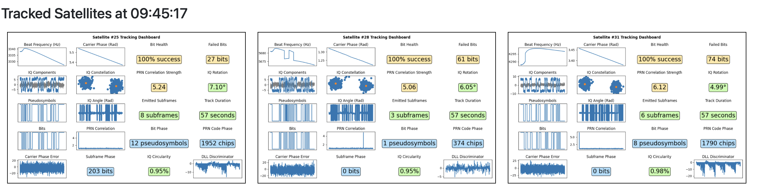
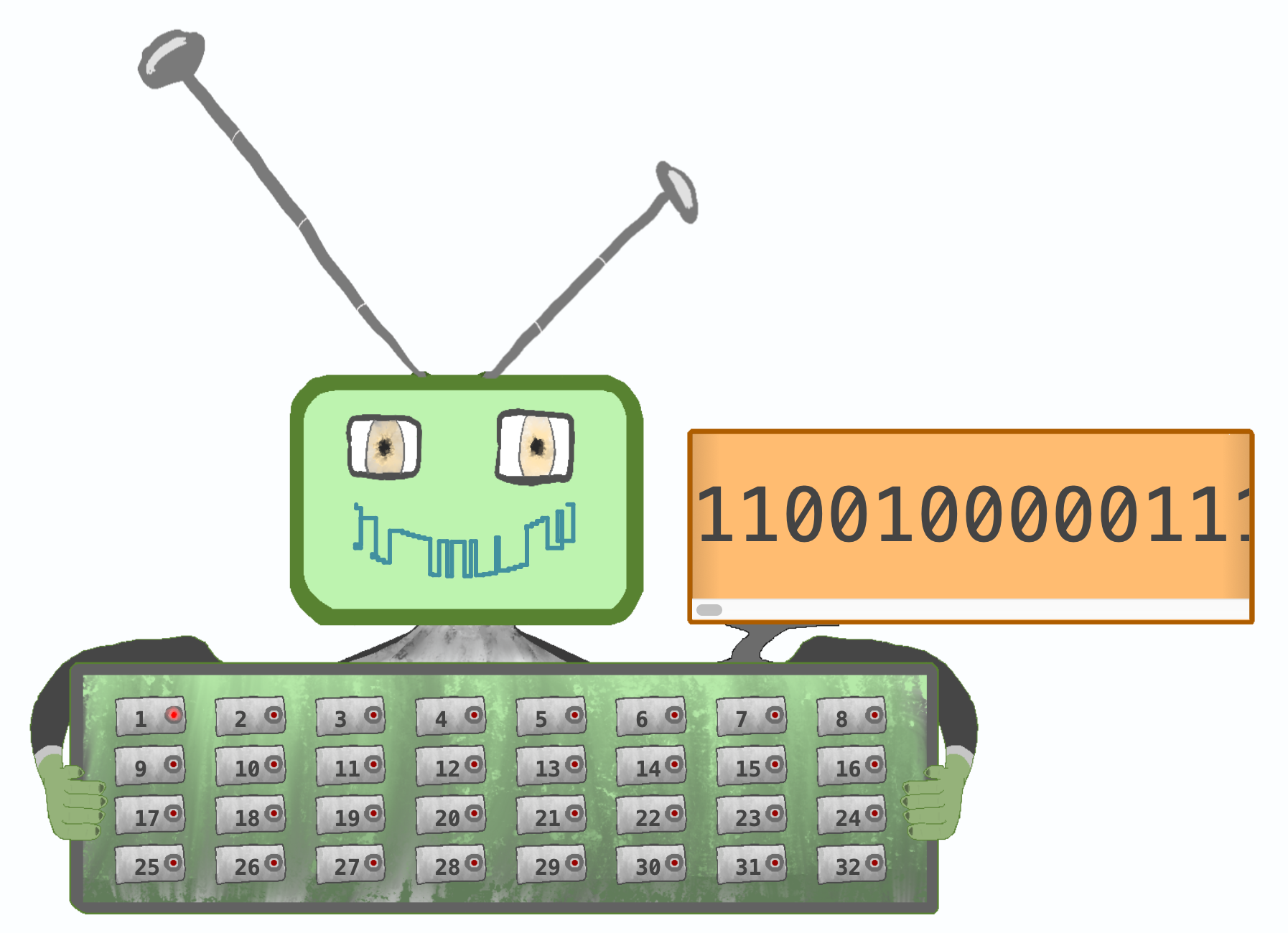
I introduced a web dashboard that communicates with the main gypsum application, and displays a dedicated satellite tracker dashboard for each satellite in view. This dashboard also displays key statistics about the GPS receiver as a whole, such as cataloguing the satellites that we’ve determined are definitely not in view, and showing some counters to denote how much of the navigation data we’ve recovered from the signals beamed down by our tracked satellites.

The satellite data

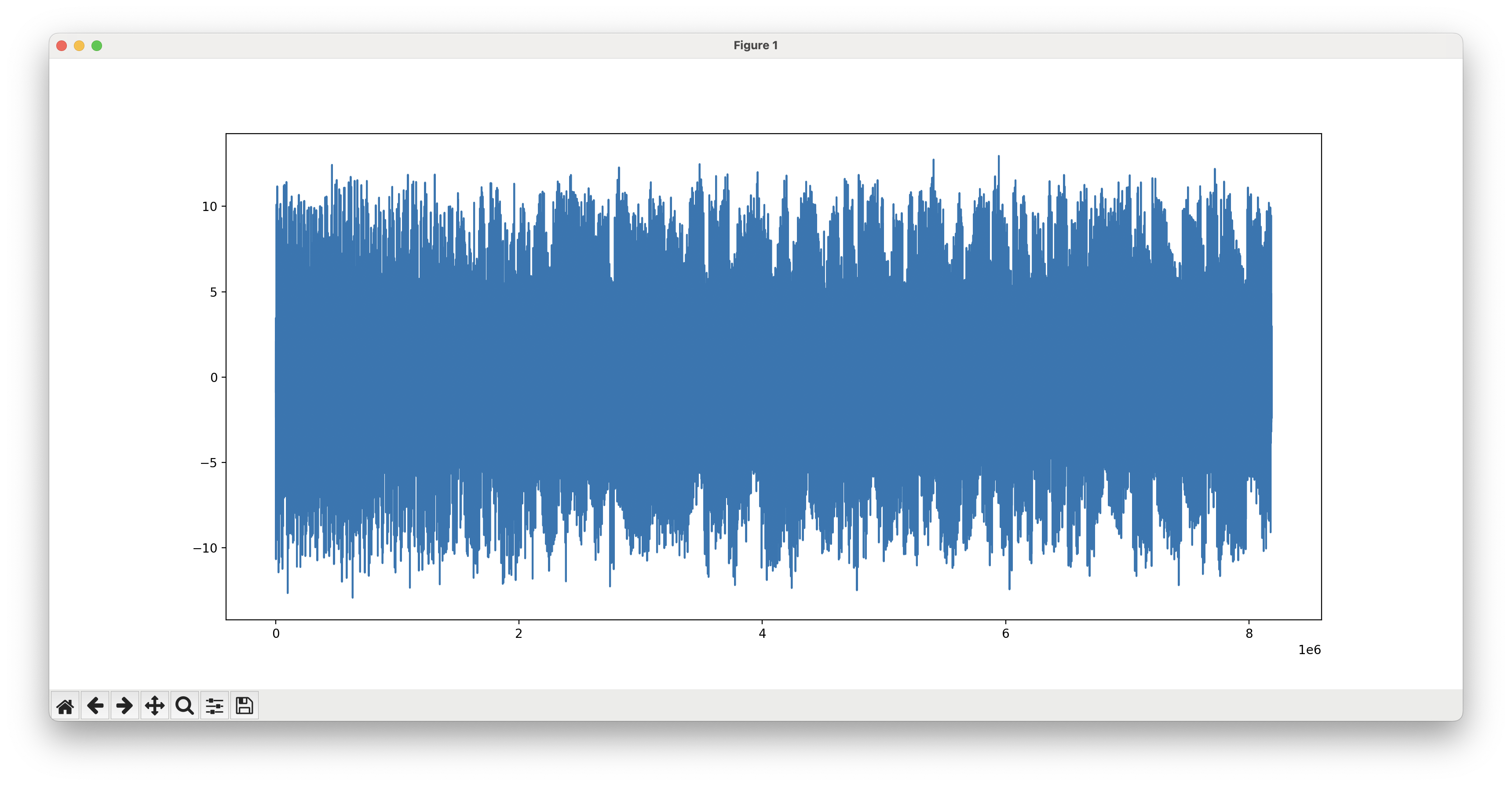
At first, it doesn’t look like much.

As our tracking loop improves, things look a bit more coherent at the start, then devolve towards the right.

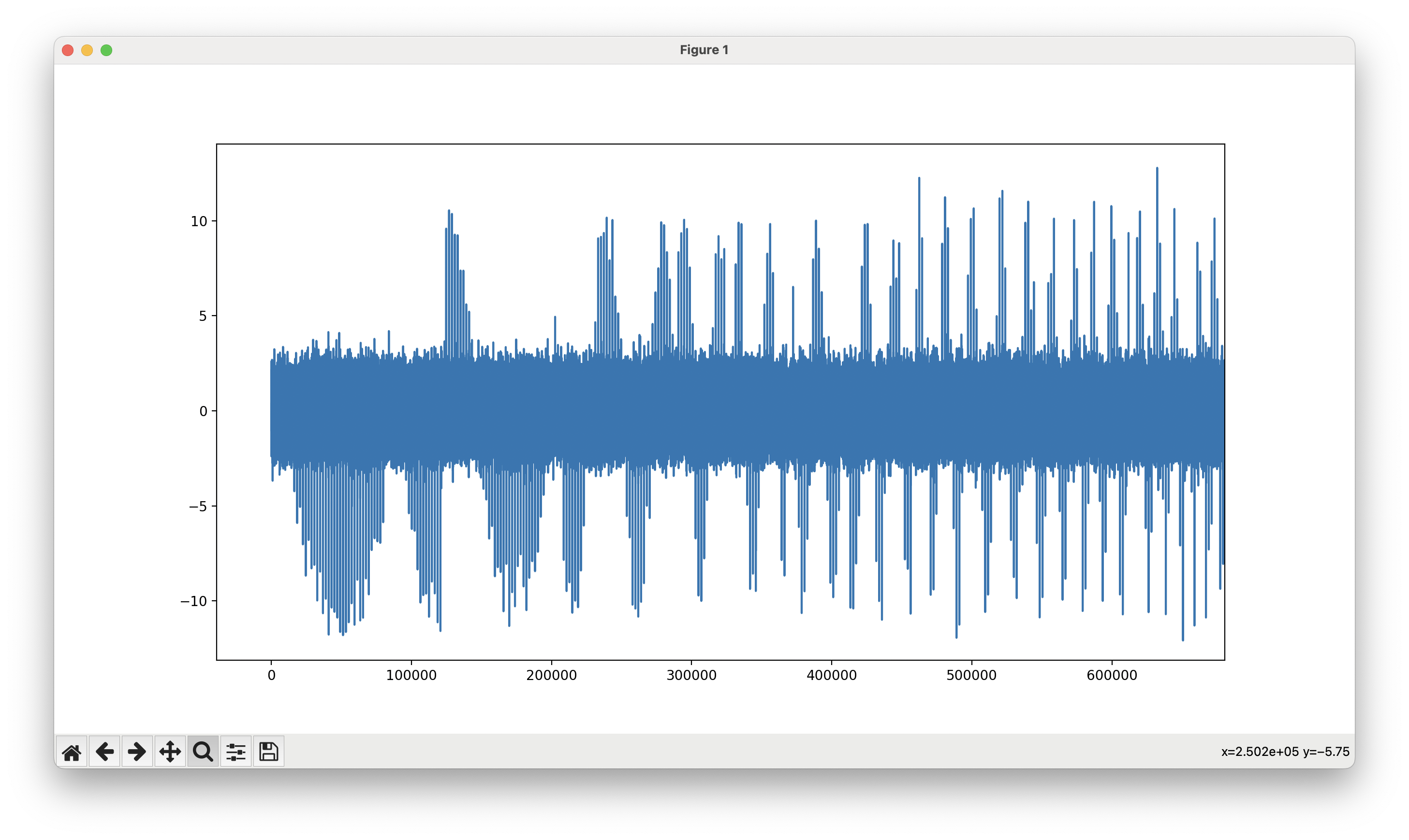
Slowly, painstakingly, the peaks become more cohesive.

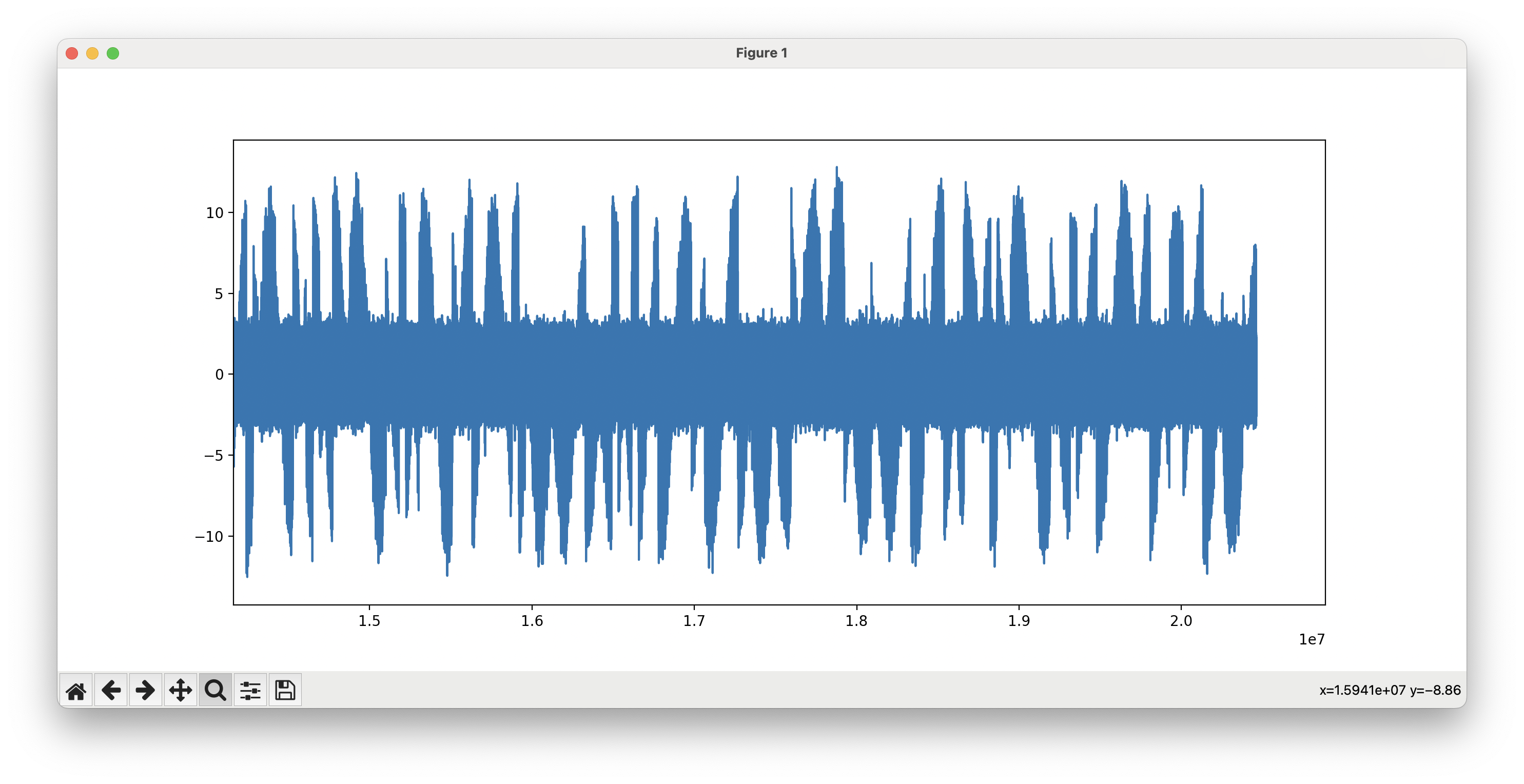
Until, finally, we have our demodulated signal!

We’re nearly ready to decode the satellite message! Read more in Part 3: Juggling Signals.